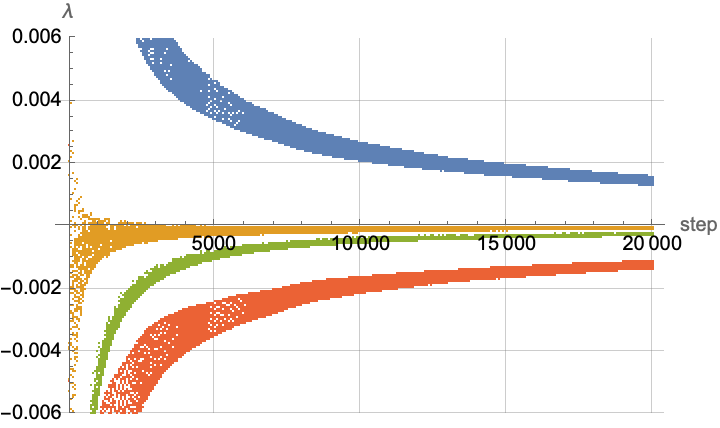
I am trying to reproduce the convergence plot of the four Lyapunov exponents for a string from this paper (page 12, figure 7).
The code that I have used till now to find the equations is given below:
K1 = 6.90; K2 = 16.05; K3 = 9.65; K4 = 3.27; K5 = 6.55;
\[Omega]sq[0] = -0.923; \[Omega]sq[1] = 6.478;
lagrangian =
  Sum[c[n]'[t]^2 - c[n][t]^2 \[Omega]sq[n], {n, {0, 1}}] +
   K1 c[0][t]^3 + K2 c[0][t] c[1][t]^2 + K3 c[0][t] c[0]'[t]^2 +
   K4 c[0][t] c[1]'[t]^2 + K5 c[0]'[t] c[1][t] c[1]'[t];
c[0][t_] := OverTilde[c][0][t] + \[Alpha]1*OverTilde[c][0][t]^2 + \[Alpha]2*OverTilde[c][1][t]^2;
c[1][t_] := OverTilde[c][1][t] + \[Alpha]3*OverTilde[c][0][t]*OverTilde[c][1][t];
\[Alpha]1 = -2; \[Alpha]2 = -0.5; \[Alpha]3 = -1;
n = Expand[lagrangian];
vars = {OverTilde[c][0][t], OverTilde[c][1][t],
   Derivative[1][OverTilde[c][0]][t],
       Derivative[1][OverTilde[c][1]][t]};
lagrangian =
  Normal[Series[n /. Thread[vars -> m*vars], {m, 0, 3}]] /. m -> 1;
momentum[n_] := D[lagrangian, Derivative[1][OverTilde[c][n]][t]]
hamiltonian = Expand[Sum[momentum[n]*Derivative[1][OverTilde[c][n]][t], {n, {0, 1}}] - lagrangian];
eulerLagrange[lagrangian_, vars_, dvars_] :=
       Thread[Table[D[D[lagrangian, dvar], t], {dvar, dvars}] - Table[D[lagrangian, var], {var, vars}] ==
         ConstantArray[0, Length[vars]]];
    equationsOfMotion = eulerLagrange[lagrangian, {OverTilde[c][0][t], OverTilde[c][1][t]},
        {Derivative[1][OverTilde[c][0]][t], Derivative[1][OverTilde[c][1]][t]}]


NDSolveon it own, due to stiffness. Did you manage to numerically solve your system? What are the initial conditions? $\endgroup$NDSolveto work on the model? Before calculating the Lyapunov exponents, you should be able to solve the dynamics. $\endgroup$