29
$\begingroup$

Does anyone know a (simple) Mathematica code for computing the Lyuponov Exponent for the Rossler System?

Thank you

Rossler System:

rossler = {

 x'[t] == -(y[t] + z[t]),

 y'[t] == x[t] + 0.1 y[t],

 z'[t] == 0.2 + x[t] z[t] - 5.7 z[t],

 x[0] == 1, y[0] == 1, z[0] == 1

}
$\endgroup$
4
  • 1
    $\begingroup$ user5267, please read this: mathematica.stackexchange.com/editing-help $\endgroup$
    – Mr.Wizard
    Commented Jan 11, 2013 at 6:45
  • $\begingroup$ @Mr.Wizard, Thank you for your help. But I really do not know what to do with this link. Can you please explain more about it? $\endgroup$
    – user5267
    Commented Jan 11, 2013 at 9:52
  • 2
    $\begingroup$ It is a guide to properly formatting your posts here on StackExchange. Well formatted questions consistently get more attention and better answers, as well as reduce the burden on those who try to clean up poorly formatting posts. There is also a "tool bar" above each edit box with a series of icons that can be used for formatting (for example, select your code and click the { } icon). $\endgroup$
    – Mr.Wizard
    Commented Jan 11, 2013 at 10:07
  • $\begingroup$ Oh. Thanks. It would be helpful. $\endgroup$
    – user5267
    Commented Jan 11, 2013 at 10:41

4 Answers 4

29
$\begingroup$

You can use the LCE package by Dr Sandri Marco. It is updated for version 7 and I just tried in on your system for V9 and it worked.

Download lcm.zip and use the package as instructed

Here is the result of running your system on it on my PC

<< lce.m

?LCEsC

Mathematica graphics

These are the 3 Lyapunov Exponents for the Rossler system:

rossler[{x_, y_, z_}] := {-y - z, x +0.1 y, 0.2 + z (x - 5.7)};
x0 = {1,1,1};
T = 0.2; K = 2000; TR = 1;  stepsize = 0.001;
lcesrossler = LCEsC[rossler, x0, T, K, TR, stepsize ]
LyapunovDimension[First[lcesrossler]]
T = 100; TR = 20;
PhaseSpaceC[rossler, x0, T, TR, stepsize, {1, 2, 3}]

giving:

{0.0647984, 0.00535441, -5.23912}

These are close to the known values for this system as given at Prof Sprott site where he has done research in this. From the above page:

Lyapunov exponents (base-e): = 0.0714, 0, -5.3943

By changing the computation parameters and if you have more time to wait, the result can be improved more to become closer to the known values.

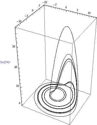
Mathematica graphics

$\endgroup$
2
  • 1
    $\begingroup$ Yes, this package is golden! Its awesome. $\endgroup$
    – dearN
    Commented Feb 6, 2016 at 22:11
  • $\begingroup$ How to use this package when ths sistem is driven. I mean the system have a equation like this x'[t]==-(y[t]+z[t])+Exp[I*t]. Can I use this package directly? $\endgroup$
    – 小菜220
    Commented Jun 6, 2016 at 8:58
28
$\begingroup$

Update May 3, 2022: Added c, i, j as local variables

Update Mar 12, 2022: Fixed mistake in implementation of PlotExponents

Update Apr 27, 2020: Got rid of AppendTo and added PlotExponents and PlotOpts options.

Update Nov 6, 2018: Tweaked to work on nonautonomous systems, to fix problem reported here.

Here's an updated implementation (works with MMA v11) that generalizes Housam Binous & Nasri Zakia's update to Marco Sandri's package and incorporates ideas from @bbgodfrey. The main advantage is that it uses NDSolve rather than Euler's method for solving the differential equations, so it should be more accurate / faster than Sandri's implementation.

First, define @halirutan's GramSchmidt:

GramSchmidt[w_?MatrixQ] := Module[{v = ConstantArray[0, Length[w]]}, 
  Table[v[[n]] = w[[n]] - Sum[(v[[i]].w[[n]]/v[[i]].v[[i]])*v[[i]], {i, n - 1}], {n, Length[w]}];
  v]

Then the main function:

LyapunovExponents[eqnsin_List, icsin : ({__Rule} | _Association), nlein_Integer: 0, opts___?OptionQ] := Module[{

(* options *)
tstep, maxsteps, ndsolveopts, logbase, showplot, plotexponents, plotopts,

(* iterators *)
c, i, j,

(* other variables *)
δ, neq, nle, vars, rhs, jac, eqns, unks, ics, cum, res, edat, state, newstate, sol, W, norms},
   
(* parse options *)
tstep = Evaluate[TStep /. Flatten[{opts, Options[LyapunovExponents]}]];
maxsteps = Evaluate[MaxSteps /. Flatten[{opts, Options[LyapunovExponents]}]];
ndsolveopts = Evaluate[NDSolveOpts /. Flatten[{opts, Options[LyapunovExponents]}]];
logbase =Evaluate[LogBase /. Flatten[{opts, Options[LyapunovExponents]}]];
showplot = Evaluate[ShowPlot /. Flatten[{opts, Options[LyapunovExponents]}]];
plotexponents = Evaluate[PlotExponents /. Flatten[{opts, Options[LyapunovExponents]}]];
plotopts = Evaluate[PlotOpts /. Flatten[{opts, Options[LyapunovExponents]}]];
  
neq = Length[eqnsin];
If[nlein == 0, nle = neq, nle = nlein]; (* how many exponents *)
   
(* extract vars and right hand sides from eqnsin *)
vars = eqnsin[[All, 1, 0, 1]];
rhs = eqnsin[[All, 2]];
   
(* jacobian matrix *)
jac = D[rhs, {Replace[vars, {x_ -> x[t]}, 1]}];
   
eqns = Join[
  eqnsin,
  Flatten[Table[δ[i, j]'[t] == (jac.Table[δ[i, j][t], {i, neq}])[[i]], {j, nle}, {i, neq}]]
];
unks = Join[
  vars,
  Flatten[Table[δ[i, j], {j, nle}, {i, neq}]]
];
ics = Join[
  Table[var[0] == (var /. icsin), {var, vars}],
  Flatten[Table[δ[i, j][0] == IdentityMatrix[neq][[i, j]], {j, nle}, {i, neq}]]
];

cum = Table[0, {nle}];

state = First@NDSolve`ProcessEquations[Flatten[Join[eqns, ics]], unks, t, Evaluate[Sequence @@ ndsolveopts]];

(* main loop *) 

edat = Table[
  newstate = First@NDSolve`Reinitialize[state, ics];
  NDSolve`Iterate[newstate, c tstep];
  sol = NDSolve`ProcessSolutions[newstate];

  W = GramSchmidt[Evaluate[Table[δ[i, j][c tstep], {j, nle}, {i, neq}] /. sol]];
  norms = Map[Norm, W];

  (* update running vector magnitudes *)
  cum = cum + Log[logbase, norms];

  ics = Join[
    Table[var[c tstep] == (var[c tstep] /. sol), {var, vars}],
    Flatten[Table[δ[i, j][c tstep] == (W/norms)[[j, i]], {j, nle}, {i, neq}]]
  ];
  cum/(c tstep)
, {c, maxsteps}];
   
If[showplot, Print[ListPlot[Transpose[edat][[1 ;; plotexponents]], Evaluate[Sequence @@ plotopts]]]];
   
Return[cum/(maxsteps tstep)]
];

Options[LyapunovExponents] = {NDSolveOpts -> {}, TStep -> 1, MaxSteps -> 10^4, LogBase -> E,
  ShowPlot -> False, PlotExponents -> 1, PlotOpts -> {}};

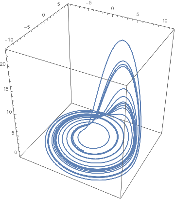
Now, onto the Rössler system. Note, the constant 0.1 in OP's equations should be 0.2 to match Sprott's results (otherwise the system is not chaotic). Let's look at the attractor.

eqns = {x'[t] == -(y[t] + z[t]), y'[t] == x[t] + 0.2 y[t],
  z'[t] == 0.2 + z[t] (x[t] - 5.7)};
sol = NDSolve[{eqns, {x[0] == 1, y[0] == 1, z[0] == 1}}, {x, y, z}, {t, 0, 1000}][[1]];
ParametricPlot3D[{x[t], y[t], z[t]} /. sol, {t, 900, 1000},  PlotRange -> All]
Mathematica graphics

Now, use the final values to start LyapunovExponents.

ics = {x -> 0.785, y -> -4.34, z -> 0.036};
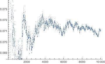
LyapunovExponents[eqns, ics, ShowPlot -> True]
Mathematica graphics

(* {0.0710707, 0.000384542, -5.39372} *)

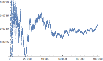
Pretty close to Sprott's values of {0.0714, 0, -5.3943} as referenced by @Nasser. If we want more accuracy, just increase MaxSteps.

LyapunovExponents[eqns, ics, ShowPlot -> True, MaxSteps -> 10^5]
Mathematica graphics

(* {0.071127, 0.0000389742, -5.39419} *)

References:

Sandri M (1996) Numerical calculation of Lyapunov exponents. The Mathematica Journal 6:78–84. https://library.wolfram.com/infocenter/Articles/2902/

Wolf A, Swift JB, Swinney HL, Vastano JA (1985) Determining Lyapunov exponents from a time series. Physica D: Nonlinear Phenomena 16:285–317. https://doi.org/10.1016/0167-2789(85)90011-9

$\endgroup$
22
  • 1
    $\begingroup$ I copied your code into Mathematica 11, but it tells me that parts of $\delta$ are undefined. I indeed see the 'other variable' $\delta$ in the function LyapunovExponents not being specified somewhere. Is it possible you forgot a line? The output of the LyapunovExponents function fails for me because it tries to evaluate Log[GramSchmidt[Norm[...]]] where the dots are the undefined components of $\delta$. $\endgroup$
    – Jeroen
    Commented Oct 3, 2018 at 19:21
  • 2
    $\begingroup$ @JgL Ugh, a semicolon was missing at the end of the line that starts jac =. Could you give it a try now? Thanks! $\endgroup$
    – Chris K
    Commented Oct 4, 2018 at 2:37
  • 2
    $\begingroup$ Note: That GramSchmidt does not provide an orthonormal basis of the span of the given list of vectors, just an orthogonal basis. (The built-in function Orthogonalize does provide an orthonormal basis -- despite its misleading name!) $\endgroup$
    – murray
    Commented Jan 9, 2019 at 16:55
  • 1
    $\begingroup$ how did you get the values of ics (x,y,z)? $\endgroup$
    – Aschoolar
    Commented Jul 3, 2021 at 13:55
  • 1
    $\begingroup$ @user444 Sorry, I have no idea. If you can define the problem in terms of a system of differential equations, you can use my LyapunovExponents function, but I'm afraid the discrete collisions will cause problems. You should ask a new question to get more eyeballs on the problem. Good luck! $\endgroup$
    – Chris K
    Commented Mar 11 at 4:45
11
$\begingroup$

Here is a sample code on how to compute the evolution of the Lyapunov Characteristic Exopnent (LCE) with Mathematica. Feel free to make any changes you like and let me know if this is what you wanted.

ClearAll["Global`*"];
deq1 = -(y1[t] + z1[t]);
deq2 = x1[t] + 0.1 y1[t];
deq3 = 0.2 + x1[t] z1[t] - 5.7 z1[t];

deq4 = -(y2[t] + z2[t]);
deq5 = x2[t] + 0.1 y2[t];
deq6 = 0.2 + x2[t] z2[t] - 5.7 z2[t];

x10 = 1; y10 = 1; z10 = 1;
dx0 = 10^-8;
x20 = x10 + dx0; y20 = y10; z20 = z10;
tin = 0; tfin = 10000;
tstep = 1;
acc = 12;

lcedata = {};
sum = 0;

d0 = Sqrt[(x10 - x20)^2 + (y10 - y20)^2 + (z10 - z20)^2 ];

For[i = 1, i < tfin/tstep, i++,

sdeq = {x1'[t] == deq1, y1'[t] == deq2, z1'[t] == deq3, 
x2'[t] == deq4, y2'[t] == deq5, z2'[t] == deq6, x1[0] == x10, 
y1[0] == y10, z1[0] == z10, x2[0] == x20, y2[0] == y20, 
z2[0] == z20};
sol = NDSolve[
sdeq, {x1[t], y1[t], z1[t], x2[t], y2[t], z2[t]}, {t, 0, tstep}, 
MaxSteps -> Infinity, Method -> "Adams", PrecisionGoal -> acc, 
AccuracyGoal -> acc];

xx1[t_]  = x1[t] /. sol[[1]];
yy1[t_]  = y1[t] /. sol[[1]];
zz1[t_] = z1[t] /. sol[[1]];

xx2[t_]  = x2[t] /. sol[[1]];
yy2[t_]  = y2[t] /. sol[[1]];
zz2[t_] = z2[t] /. sol[[1]];

d1 = Sqrt[(xx1[tstep] - xx2[tstep])^2 + (yy1[tstep] - yy2[tstep])^2 + 
          (zz1[tstep] - zz2[tstep])^2 ];

sum += Log[d1/d0];
dlce = sum/(tstep*i);
AppendTo[lcedata, {tstep*i, Log10[dlce]}];

w1 = (xx1[tstep] - xx2[tstep])*(d0/d1); 
w2 = (yy1[tstep] - yy2[tstep])*(d0/d1);
w3 = (zz1[tstep] - zz2[tstep])*(d0/d1); 

x10 = xx1[tstep];
y10 = yy1[tstep];
z10 = zz1[tstep];

x20 = x10 + w1;
y20 = y10 + w2;
z20 = z10 + w3;

i = i++;

If[Mod[tstep*i, 100] == 0, 
Print[" For t = ", tstep*i, " , ", " LCE = ", dlce]]

]

S0 = ListPlot[{lcedata}, Frame -> True, Axes -> False, 
PlotRange -> All, Joined -> True, 
          FrameLabel -> {"t", "log10(LCE)"}, 
FrameStyle -> Directive["Helvetica", 17], ImageSize -> 550]
$\endgroup$
1
  • 2
    $\begingroup$ May I ask a question? What the difference between the Lyapunov Characteristic Exopnent in this progress and the Maximal Lyapunov exponent? $\endgroup$
    – 小菜220
    Commented Jun 6, 2016 at 8:27
9
$\begingroup$

At first, let's solve the system of ODEs. Taking into account that you give specific initial conditions, then the solution of the system will correspond to a three-dimensional orbit. The following code solves the system of the ODEs and also plots the output 3D orbit. Now, about the Lyapunov Exponent. How exactly do you define this exponent. I mean, by using the variational equations or by monitoring the deviation between two initially nearby orbits? If it is the latter, then I could provide such a Mathematica code.

Clear["Global`*"];
deq1 = -(y[t] + z[t]);
deq2 = x[t] + 0.1 y[t];
deq3 = 0.2 + x[t] z[t] - 5.7 z[t];
x0 = y0 = z0 = 1;
tin = 0;
tfin = 50;
sol = NDSolve[{x'[t] == deq1, y'[t] == deq2, z'[t] == deq3, 
x[0] == x0, y[0] == y0, z[0] == z0}, {x[t], y[t], z[t]}, {t, tin, 
tfin}];
xt = x[t] /. sol[[1]];
yt = y[t] /. sol[[1]];
zt = z[t] /. sol[[1]];
P1 = ParametricPlot3D[{xt, yt, zt}, {t, tin, tfin}, 
AxesLabel -> {"x", "y", "z"}, BoxRatios -> {1, 1, 1}, 
PlotRange -> All]
$\endgroup$
2
  • $\begingroup$ Thank you for your answer.By the way, I think that these two methods almost give the same results. Aren't they?! I appreciate it, if you share your idea about it. $\endgroup$
    – user5267
    Commented Jan 11, 2013 at 9:44
  • $\begingroup$ Can you help me in computing the largest Lyapunov exponent in the case of variational equations...do we have to do analytically or computationally, please suggest some methods to compute this lyapunov exponent!. $\endgroup$
    – BAYMAX
    Commented Mar 9, 2018 at 11:13

Your Answer

By clicking “Post Your Answer”, you agree to our terms of service and acknowledge you have read our privacy policy.

Not the answer you're looking for? Browse other questions tagged or ask your own question.