Speeding up the Kuramoto model on a random graph

Question

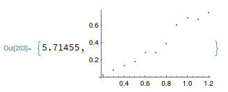
I am solving the Kuramoto model on a random graph $G(n,p)$, plotting the synchrony against the coupling parameter, as follows,

n = {300};
tmax = 100;
evaltime = 10;
SeedRandom[Nosc];
rg1 = RandomGraph[BernoulliGraphDistribution[n[[1]], 6/n[[1]]]];
rg2 = AdjacencyGraph[AdjacencyMatrix[rg1]];
Nosc = Length@VertexList[rg2];
omegadata = VertexDegree[rg2];
 \[Theta]start = RandomReal[{0, 2*Pi}, Nosc];
A = AdjacencyMatrix[rg2];
avg = 1;
a[l_, t_] := Module[{}, \[Lambda] = l;
  eqns1 = {Table[\[Theta][i]'[tt] == 
      omegadata[[i]] + \[Lambda]*
        Sum[A[[i, j]] (Sin[\[Theta][j][tt] - \[Theta][i][tt]]), {j, 1,
           Nosc, 1}], {i, 1, Nosc, 1}], 
    Table[\[Theta][i][0] == \[Theta]start[[i]], {i, 1, Nosc, 1}]};
  sol1 = NDSolve[eqns1, 
    Table[\[Theta][i], {i, 1, Nosc, 1}], {tt, 0, tmax, 1}];
  Table[Evaluate[Table[\[Theta][i][t], {i, 1, Nosc, 1}] /. sol1][[1, 
    i]], {i, 1, Nosc}]
  ]
ListPlot[Table[{i, 
    Abs[1/Nosc Total[
       Exp[-I Mean[Table[a[i, evaltime], {j, 1, avg}]]]]]}, {i, 0.2, 
    1.2, 0.1}], PlotRange -> Full] // AbsoluteTiming

It only takes 5 seconds here, but with more oscillators it can take much longer. Is it possible to get NDSolve to obtain only an approximate solution much faster by adding options (or obtain a solution using a different method)? This might help when the graph is large and the simulation takes much longer.

Answer 1

Solving the system purely numerically (without any symbolic computations) is a bit faster. This can be done by using the signed incidence matrix of the graph (matrix B below).

I have to use the \[Theta]_?VectorQ pattern in otder to prevent NDSolve from starting any symbolic analysis.

ParametricNDSolveValue provides a neat way to collect everyting into a single function.

Also, there is no point in solving the ODE until tmax if the solution is evaluated only at evaltime; so I let just return the state at that time, not the whole InterpolationFunction.

ClearAll[\[Lambda], T];
B = N[IncidenceMatrix[Graph[UpperTriangularize[A]["NonzeroPositions"],DirectedEdges -> True]]];
X[\[Theta]_?VectorQ, \[Lambda]_] := N[omegadata] - \[Lambda] B . Sin[\[Theta] . B];
newa = ParametricNDSolveValue[{
  \[Theta]'[t] == X[\[Theta][t], \[Lambda]], 
  \[Theta][0] == \[Theta]start}, \[Theta][T], 
  {t, 0, T}, {\[Lambda], T}];

aa = a[0.2, evaltime]; // AbsoluteTiming // First
bb = newa[0.2, evaltime]; // AbsoluteTiming // First
Max[Abs[aa - bb]/Max[Abs[aa]]]

1.65085

0.019422

4.63889*10^-8

This turns out to be almost 100 times faster. Probably a different ODE integrator is applied, which explains the small difference of the results.

Answer 2

There are probably other improvements to be had, but the first thing I noticed is passing a bunch of InterpolatingFunctions out from a[l,t] seems inefficient. This calculates more in a[l,t] and speeds up 3X on my computer:

a[l_, t_] := Module[{}, \[Lambda] = l;
  eqns1 = {Table[\[Theta][i]'[tt] == 
      omegadata[[i]] + \[Lambda]*
        Sum[
         A[[i, j]] (Sin[\[Theta][j][tt] - \[Theta][i][tt]]), {j, 1, 
          Nosc, 1}], {i, 1, Nosc, 1}], 
    Table[\[Theta][i][0] == \[Theta]start[[i]], {i, 1, Nosc, 1}]};
  sol1 = 
   NDSolve[eqns1, 
    Table[\[Theta][i], {i, 1, Nosc, 1}], {tt, 0, tmax, 1}];
  res = Table[\[Theta][i][t], {i, Nosc}] /. sol1[[1]];
  Abs[1/Nosc Total[Exp[-I Mean[Table[res, {j, 1, avg}]]]]]
  ]

ListPlot[Table[{i, a[i, evaltime]}, {i, 0.2, 1.2, 0.1}], 
  PlotRange -> Full] // AbsoluteTiming