10
$\begingroup$

I am working on an interesting problem, that consists of trying to compute the shortest distance between two points on a 2D surface. This 2D surface can be represented in a 3D space by the function $f(x,y)=z$. To do this, I solve the geodesic equation and compute the arc length of the solution $\{x_\text{sol}(t),y_\text{sol}(t)\}$ where $t$ will be the parameter to describe the trajectory. However when I test my solution for simple cases I get slightly wrong results and I am not sure why. Here is an example:

Generate surface and points:

f[x_, y_] := -x^2 - y^2 + 1
{x0, y0} = {0, 0};
{x1, y1} = {0, Sin[Pi/2]};
surface = 
  ContourPlot3D[f[x, y] == z, {x, -1, 1}, {y, -1, 1}, {z, 0, 2}, 
   ContourStyle -> {Yellow, Opacity[0.8]}];
ptsPlot = 
  ListPointPlot3D[{{x0, y0, f[x0, y0]}, {x1, y1, f[x1, y1]}}, 
   PlotRange -> All, PlotStyle -> {Black, PointSize[0.05]}];
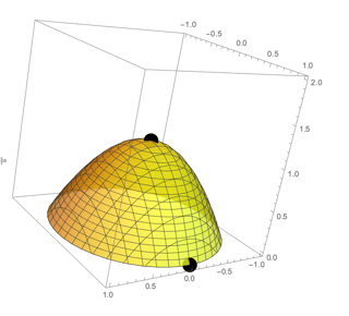
Show[surface, ptsPlot]
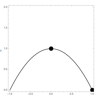
Show[ContourPlot[f[0, y] == z, {y, -1, 1}, {z, 0, 2}, 
  ContourStyle -> Black], 
 ListPlot[{{y0, f[0, y0]}, {y1, f[0, y1]}}, PlotRange -> All, 
  PlotStyle -> {Black, PointSize[0.05]}]]

enter image description here

I chose points that are aligned on the $x$-axis so that I can easily test my answer: in this case, the shortest distance will be a trajectory on the $yz$-plane. The distance will the length of the following curve:

enter image description here

Find Geodesic

Then, to solve the geodesic equation I compute the Lagragian, and use a package VariationalMethods that solves the Euler Lagrange equation for me:

Needs["VariationalMethods`"]

(*Find Lagrangian by computing the metric from the line element*)
Lagrange = (1 + D[f[x[t], y[t]], x[t]]^2)*
    x'[t]^2 + (1 + D[f[x[t], y[t]], y[t]]^2)*y'[t]^2 + 
   2*D[f[x[t], y[t]], x[t]]*D[f[x[t], y[t]], y[t]];

(*Mathematica differentiates everything and writes down the Euler \
Lagrange Equation for us*)
{eq1, eq2} = 
  EulerEquations[Lagrange, {x[t], y[t]}, {t}];

(*Solve it, nb: since we only care about the distance we can put any \
time interval*)

S = NDSolve[{eq1, eq2, x[0] == x0, x[1] == x1, y[0] == y0, 
    y[1] == y1}, {x[t], y[t]}, {t, 0, 1}];
xsol[t_] := Evaluate[x[t] /. S[[1, 1]]]
ysol[t_] := Evaluate[y[t] /. S[[1, 2]]]
solution = 
  ParametricPlot3D[{xsol[t], ysol[t], f[xsol[t], ysol[t]]}, {t, 0, 1},
    PlotRange -> All, PlotStyle -> Red];
Show[surface, solution, ptsPlot]

Verify solution

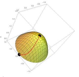
However if I plot the solution I obtain we can see that it is slightly off:

enter image description here

In fact, if I compute the error by calculating the arclength of the true trajectory, I have almost an error of almost $20\%$ :

distance = NIntegrate[ Sqrt[xsol'[t]^2 + ysol'[t]^2], {t, 0, 1}] (*Arc Length*)
(*1.19323*)
trueDistance = ArcLength[1 - y^2, {y, 0, 1}] // N
(*1.47894*)

Which is not desirable at all. How could I improve this method? What am I doing wrong?

Edit:

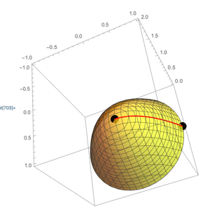
Daniel Huber's comment made the trick: now it works really well! here is the plot of solution for the example I used:

Needs["VariationalMethods`"]

(*Find Lagrangian by computing the metric from the line element*)
Lagrange = Module[{}, z = f[x[t], y[t]]; r = {x[t], y[t], z};
   ds = Sqrt[D[r, t] . D[r, t]];
   ds*ds
   ];
Print["Lagrange=", Lagrange]
(*Mathematica differentiates everything and writes down the Euler \
Lagrange Equation for us*)
{eq1, eq2} = EulerEquations[Lagrange, {x[t], y[t]}, {t}];

(*Solve it,nb:since we only care about the distance we can put any \
time interval*)

S = NDSolve[{eq1, eq2, x[0] == x0, x[1] == x1, y[0] == y0, 
    y[1] == y1}, {x[t], y[t]}, {t, 0, 1}];
xsol[t_] := Evaluate[x[t] /. S[[1, 1]]]
ysol[t_] := Evaluate[y[t] /. S[[1, 2]]]
zsol[t_] := Evaluate[f[xsol[t], ysol[t]]];
solution = 
  ParametricPlot3D[{xsol[t], ysol[t], f[xsol[t], ysol[t]]}, {t, 0, 1},
    PlotRange -> All, PlotStyle -> Red];
Show[surface, solution, ptsPlot]
distance = 
 NIntegrate[Sqrt[xsol'[t]^2 + ysol'[t]^2 + zsol'[t]^2], {t, 0, 1}] // 
  NumberForm[#, 10] &(*Arc Length*)

enter image description here

Second Edit:

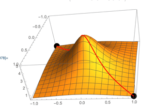
I found examples where this notebook fails to give me the shortest distance, for example use:

(* Define Surface*)
f[x_, y_] := 1/(x^2 + y^2 + 0.2)
surface = Plot3D[f[x, y], {x, -1, 1}, {y, -1, 1}];

(*Determine points*)
{x0, y0} = {-1, -1};
{x1, y1} = {1, 1};
ptsPlot = 
  ListPointPlot3D[{{x0, y0, f[x0, y0]}, {x1, y1, f[x1, y1]}}, 
   PlotRange -> All, PlotStyle -> {Black, PointSize[0.05]}];
Show[surface, ptsPlot]

enter image description here

This tells me that the trajectory is by climbing the summit of the mountain, which must be clearly wrong. Is this an error in the NDSolve?

$\endgroup$
8
  • 5
    $\begingroup$ I think your line element is wrong. It should be Sqrt[D[r,t].D[r,t]] where r is the position vectors of the surface: r= {x[t],y[t],f[x[t],y[t]]} $\endgroup$ Commented Dec 6, 2021 at 9:48
  • $\begingroup$ It works incredibly well now, thank you! Do you have a link or reference that explains why the line element is Sqrt[D[r,t].D[r,t]] ? What happens in the case where I have a closed surface? $\endgroup$
    – Matt
    Commented Dec 6, 2021 at 14:07
  • 2
    $\begingroup$ It is no magic, only simple math: if r[t] is a position vector dependent on t, then an infinite increment is : ds= D[r[t],t] . dt. And the length of the infinite increment, the line element, is: Sqrt[ds.ds]= Sqrt[r'.r'] dt. This will also work on closed surfaces. $\endgroup$ Commented Dec 6, 2021 at 14:26
  • 4
    $\begingroup$ The Euler Lagrange equation gives you stationary path. That is small changes do not change the pathlength in linear approximation. Therefore, you can get a maximal path as well as a minimal one. Try perturbing the initial stat a bit. $\endgroup$ Commented Dec 7, 2021 at 8:55
  • 1
    $\begingroup$ Try calculating the pathlength with a middle point that is not exactly on the original path and check if the pathlength decreases. $\endgroup$ Commented Dec 7, 2021 at 9:24

1 Answer 1

3
$\begingroup$

This answer is for the second editing of the question.

The variational method provides an extreme value, which can of course be a maximum value.NDSolvecan only give one solution of equations. You can change the starting initial condition of Shooting method to get other solutions.

Use Method -> {"BoundaryValues" -> {"Shooting", StartingInitialConditions" -> {x'[0] == 0}}} for NDSolve as

Needs["VariationalMethods`"]

f[x_, y_] := 1/(x^2 + y^2 + 0.2)
surface = Plot3D[f[x, y], {x, -1, 1}, {y, -1, 1}];

(*Determine points*)
{x0, y0} = {-1, -1};
{x1, y1} = {1, 1};
ptsPlot = ListPointPlot3D[{{x0, y0, f[x0, y0]}, {x1, y1, f[x1, y1]}}, PlotRange -> All, PlotStyle -> {Black, PointSize[0.05]}];
(*Find Lagrangian by computing the metric from the line element*)
Lagrange = Module[{}, 
    z = f[x[t], y[t]]; 
    r = {x[t], y[t], z};
    ds = Sqrt[D[r, t] . D[r, t]];
    ds*ds];
Print["Lagrange=", Lagrange]
(*Mathematica differentiates everything and writes down the Euler-Lagrange Equation for us*)
{eq1, eq2} = EulerEquations[Lagrange, {x[t], y[t]}, {t}];

(*Solve it,nb:since we only care about the distance we can put any time interval*)
s1 = NDSolve[{eq1, eq2, x[0] == x0, x[1] == x1, y[0] == y0, y[1] == y1}, {x[t], y[t]}, {t, 0, 1}];
s2 = NDSolve[{eq1, eq2, x[0] == x0, x[1] == x1, y[0] == y0, y[1] == y1}, {x[t], y[t]}, {t, 0, 1}, Method -> {"BoundaryValues" -> {"Shooting", "StartingInitialConditions" -> {x'[0] == 0}}}]
x1sol[t_] := Evaluate[x[t] /. s1[[1, 1]]];
y1sol[t_] := Evaluate[y[t] /. s1[[1, 2]]]
z1sol[t_] := Evaluate[f[x1sol[t], y1sol[t]]];
solution1 = ParametricPlot3D[{x1sol[t], y1sol[t], f[x1sol[t], y1sol[t]]}, {t, 0,1}, PlotRange -> All, PlotStyle -> Red];
x2sol[t_] := Evaluate[x[t] /. s2[[1, 1]]]
y2sol[t_] := Evaluate[y[t] /. s2[[1, 2]]]
z2sol[t_] := Evaluate[f[x1sol[t], y1sol[t]]];
solution2 = ParametricPlot3D[{x2sol[t], y2sol[t], f[x2sol[t], y2sol[t]]}, {t, 0, 1}, PlotRange -> All, PlotStyle -> Blue];
Show[surface, solution1, solution2, ptsPlot]
distance1 = NIntegrate[Sqrt[x1sol'[t]^2 + y1sol'[t]^2 + z1sol'[t]^2], {t, 0, 1}] // NumberForm[#, 10] &
distance2 = NIntegrate[Sqrt[x2sol'[t]^2 + y2sol'[t]^2 + z2sol'[t]^2], {t, 0, 1}] // NumberForm[#, 10] &

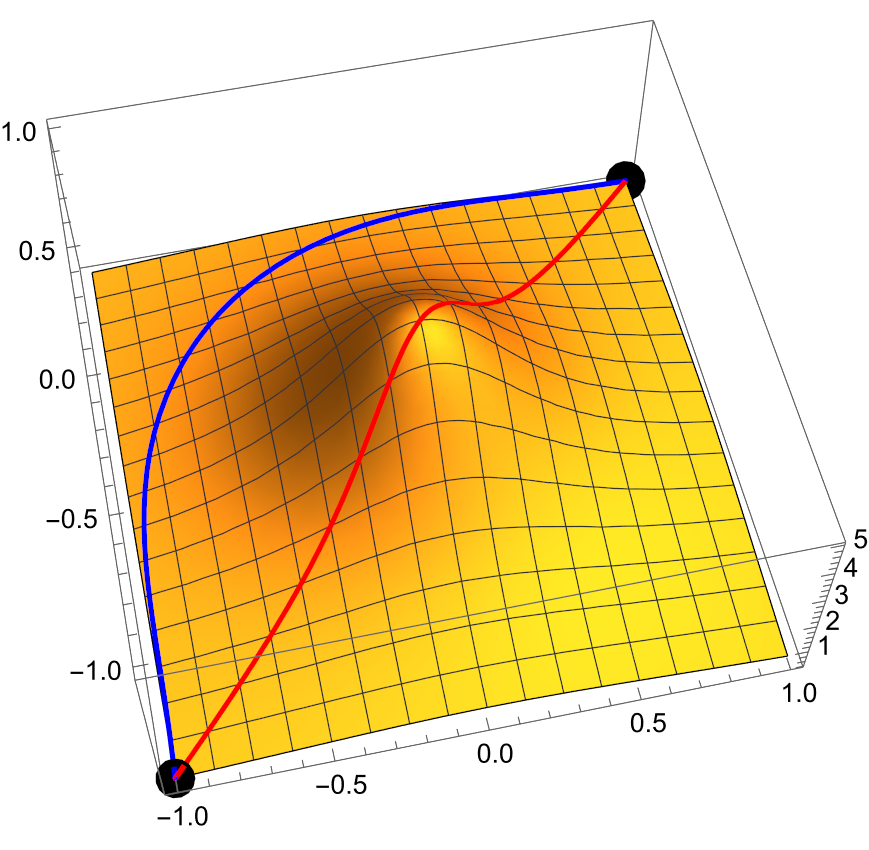
you will get red line for s1 and blue line for s2. enter image description here

The distance for red is 9.780379488 and for blue line is 9.724140753.

$\endgroup$
2
  • 3
    $\begingroup$ Please post the Mathematica code. $\endgroup$
    – cvgmt
    Commented May 31 at 8:03
  • $\begingroup$ My code only sets methods based on the code in the problem, so I didn't show it at the beginning. If you wish, I will post it. $\endgroup$
    – houzw
    Commented May 31 at 10:28

Your Answer

By clicking “Post Your Answer”, you agree to our terms of service and acknowledge you have read our privacy policy.

Not the answer you're looking for? Browse other questions tagged or ask your own question.