Problem with NDSolve regarding initial conditions of the derivative of a parametric function

Question

I have a function functiontoplot defined using the following piece of code:

f1 = -α*u*v + u*(1 - u)*(u - m)*(u + v);
f2 = β*u*v - γ*v*(u + v);
eq = Solve[{f1, f2} == 0, {u, v}][[5]];
jacobianmat = D[{f1, f2}, {{u, v}}];
diffmatrix = DiagonalMatrix[{D1, D2}];
det = Simplify[Det[jacobianmat - μ*diffmatrix] /. eq];
der = Simplify[D[det, μ]];
ksquared = Simplify[Solve[der == 0, μ][[1]]];
functiontoplot = Simplify[det /. ksquared];
α = 0.24;
β = 0.19;
γ = 0.01;
D2 = 10^-4;

With this, functiontoplot depends on two parameters: $m$ and $D1$. I want to plot the implicit curve defined by the equation functiontoplot==0, using the method of pseudo-arclength continuation. Up until now, I have tried with the following piece of code:

func = functiontoplot /. {m -> m[t], D1 -> D1[t]};
eqn = D[func, t] == 0;
D1values = D1 /. Quiet@Solve[functiontoplot == 0 /. m -> 0.0461, D1];
sol = NDSolve[{eqn, m'[t]^2 + D1'[t]^2 == 1, m[0] == 0.0461, D1[0] == D1values[[1]]}, {m, D1}, {t, -15, 15}

but after running it, I get the following error:

With that in mind, I tried changing the last line of the previous code by

sol = NDSolve[{eqn, m'[t]^2 + D1'[t]^2 == 1, m[0] == 0.0461, D1[0] == D1values[[1]]}, {m, D1}, {t, -15, 15}, Method -> {"EquationSimplification" -> "Residual"}];

But I get the following output:

Is there a way to estimate the derivatives of the functions $m[t]$ and $D1[t]$, or another method to solve this problem?

I have plotted the curve using the following line of code:

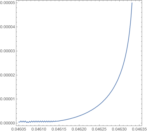
ContourPlot[functiontoplot == 0, {m, 0.04605, 0.04635}, {D1, 0, 0.00005}]

and I have gotten the following output:

Yet I want to be able to plot the function in an accurate way using the pseudo-arclength continuation method to plot other curves that may be defined by messy functions that ContourPlot takes a long time to plot.

Answer 1

I could solve my problem using a different approach. There are four equations that determine the variable eqn. Using these expressions as different equations instead of combining them is a better idea when using NDSolve.

The first part of the code is quite similar. I only removed the evaluations in the variables eq and ksquared in det and functiontoplot, respectively. Also, I changed the name of functiontoplot to auxiliarequation. In particular, I used the following piece of code:

f1 = -α*u*v + u*(1 - u)*(u - m)*(u + v);
f2 = β*u*v - γ*v*(u + v);
eq = Solve[{f1, f2} == 0, {u, v}][[5]];
jacobianmat = D[{f1, f2}, {{u, v}}];
diffmatrix = DiagonalMatrix[{D1, D2}];
det = Simplify[Det[jacobianmat - μ*diffmatrix]];
der = Simplify[D[det, μ]];
ksquared = Simplify[Solve[der == 0, μ][[1]]];
auxiliarequation = Simplify[det /. ksquared /. eq];
α = 0.24;
β = 0.19;
γ = 0.01;
D2 = 10^-4;
f1aux = f1 /. m -> m[t] /. D1 -> D1[t] /. μ -> μ[t] /. 
    u -> u[t] /. v -> v[t];
f2aux = f2 /. m -> m[t] /. D1 -> D1[t] /. μ -> μ[t] /. 
    u -> u[t] /. v -> v[t];
auxdet = det /. m -> m[t] /. D1 -> D1[t] /. μ -> μ[t] /. 
    u -> u[t] /. v -> v[t];
auxder = der /. m -> m[t] /. D1 -> D1[t] /. μ -> μ[t] /. 
    u -> u[t] /. v -> v[t];
f1aux = D[f1aux, t];
f2aux = D[f2aux, t];
auxdet = D[auxdet, t];
auxder = D[auxder, t];

Also, as you can see, I defined new variables that are part of the parametrized curve. The only things that are missing are the initial conditions and, of course, the integration of the system. For that purpose, I used the following piece of code:

initialm = 0.04615;
initialD1 = 
  D1 /. Quiet@FindRoot[auxiliarequation /. m -> initialm, {D1, 10^-6}];
initialμ = 
  ksquared[[1]][[2]] /. eq /. m -> initialm /. D1 -> initialD1;
initialeq = eq /. m -> initialm /. D1 -> initialD1;
sol = Quiet@
   NDSolve[{f1aux == 0, f2aux == 0, auxdet == 0, auxder == 0, 
     m'[t]^2 + D1'[t]^2 + μ'[t]^2 + u'[t]^2 + v'[t]^2 == 100, 
     m[0] == initialm, D1[0] == initialD1, μ[0] == initialμ, 
     u[0] == initialeq[[1]][[2]], v[0] == initialeq[[2]][[2]]}, {m[t],
      D1[t], μ[t], u[t], v[t]}, {t, -1000, 1000}, 
    Method -> {"EquationSimplification" -> "Residual"}];

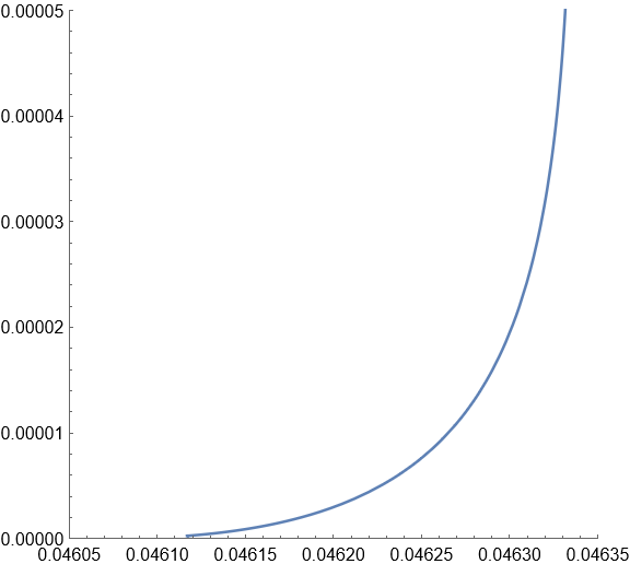
Finally, after using the classical ParametricPlot with this command line:

ParametricPlot[{m[t], D1[t]} /. sol[[1]], {t, -1000, 1000}, 
 AspectRatio -> 1, PlotRange -> {{0.04605, 0.04635}, {0, 0.00005}}]

we get the following output: