NonStandard finite difference for BMBB equation

Question

I am trying to implement the following scheme mentioned in the paper

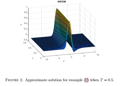
"NUMERICAL SOLUTIONS OF BENJAMIN-BONA-MAHONY-BURGERS EQUATION VIA NONSTANDARD FINITE DIFFERENCE SCHEME " What is mentioned in the paper for the BMMB Equation : http://math-frac.org/Journals/EJMAA/Vol6(2)_July_2018/Vol6(2)_Papers/21_EJMAA_Vol6(2)_July_2018_pp_237-245.pdf

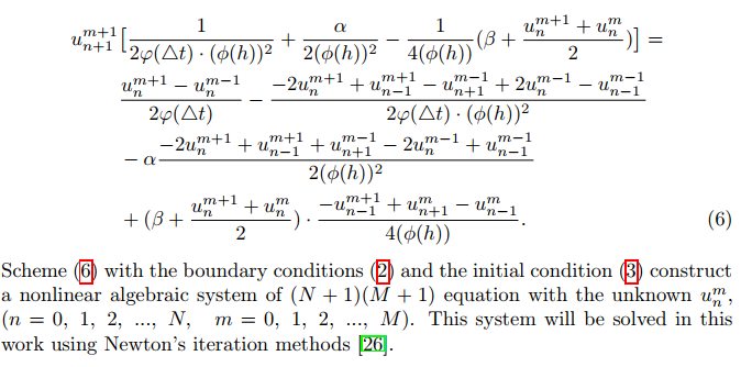
Using the following scheme

I have tried this code in Mathematica

How to discretize a nonlinear PDE fast? nonlinear-pde-fast/28011 Code Edited following the post

NN = 8 ;
M = 8 ;
a = -10 ; 
b = 10 ;
h = (b - a)/NN;
T = 0.5 ;
k = T/M ; 
\[Phi][x_] = (E^(Sqrt[2] h/3) - 2 + E^(-Sqrt[2] h/3))/(2/9);
\[Psi][y_] = Sinh[y];
(*Defining the Grid points*)
Table[Subscript[x,i] = -10 + i h , {i , 0, M}];
Table[Subscript[t,j] = 0 + j k , {j , 0 , NN } ] ;
(*Defining the Initial Conditions*)
For[i = 0, i <= M, i++ ,Subscript[w , i , 0 ] = E^(-Subscript[x, i]*Subscript[x, i])];
(*Defining the Boundary Conditions*)
For [j = 0 , j <= NN , j++, Subscript[w, 0, j]  = 0];

For[j = 0 , j <= NN , j++ ,Subscript[w, M, j]  = 0];

(*Defining the nonlinear equations due to discritization*)
For[i = 1 , i <= NN, 
  i++ , {For [j = 1, j <= M - 1 , j++, 
    f[i, j] = 
     Subscript[w, i + 1, 
        j + 1]*(1/(2*\[Psi][k]*(\[Phi][h])^2) + 1/(
         2 *(\[Phi][h])^2) - 
         1/(4*\[Phi][h])*(1 + (
            Subscript[w, i, j + 1] + Subscript[w, i, j])/2))
      - ((Subscript[w, i, j + 1] - Subscript[w, i, j - 1])/(
        2* \[Psi][k]) - (-2 *Subscript[w, i, j + 1] + 
         Subscript[w, i - 1, j + 1] - Subscript[w, i + 1, j - 1] + 
         2*Subscript[w, i, j - 1] - Subscript[w, i - 1, j - 1])/(
        2* \[Psi][k]*(\[Phi][h])^2)
        - (-2*Subscript[w, i, j + 1] + Subscript[w, i - 1, j + 1] + 
         Subscript[w, i + 1, j - 1] - 2*Subscript[w, i, j - 1] + 
         Subscript[w, i - 1, j - 1])/(2*(\[Phi][h])^2
        )
        + (1 + (Subscript[w, i, j + 1] + Subscript[w, i, j])/
           2)*((-Subscript[w, i - 1, j + 1] + Subscript[w, i + 1, j] -
            Subscript[w, i - 1, j])/(4*(\[Phi][h]))))]}];
Sys = Flatten[Table[f[i, j], {i, M - 1}, {j, NN }]]//FullSimplify;

Vec = Flatten[Table[Subscript[w, i, j], {i, M - 1}, {j, NN}]];
Sol = FindRoot[Sys, {#, 1} & /@ Vec]

I get an error with FindRoot
How can i fix my code to show the result For N=M=8 ?

Answer 1

As it mentioned by xzczd we need to add some initial condition to this model. In a case of Example 2 we can use for example $u_t=0$ at $t=0$, then we have

u0[x_] := Exp[-x^2]; u1[x_] := 0;ue[x_,t_]:=0;
a = -10;
b = 10; NN = 200;
M = 50; alpha = 1; beta = 1; c = 1/10; v = 1 + c; kap = Sqrt[c/(4 v)];
h = (b - a)/NN; xcol = Table[a + h i, {i, 0, NN}];
T = 1/2; dt = T/M; tcol = Table[dt j, {j, 0, M}];
\[Phi][x_] := (E^(Sqrt[2] x/3) - 2 + E^(-Sqrt[2] x/3))/(2/9);
\[Psi][y_] := Sinh[y];




    eqn = Table[(u[n, m + 1] - u[n, m - 1])/(2 \[Psi][dt]) - (u[n + 1, m + 1] - 
    2 u[n, m + 1] + u[n - 1, m + 1] - u[n + 1, m - 1] + 
    2 u[n, m - 1] - u[n - 1, m - 1])/(2 \[Psi][dt] \[Phi][h]) - 
 alpha (u[n + 1, m + 1] - 2 u[n, m + 1] + u[n - 1, m + 1] + 
     u[n + 1, m - 1] - 2 u[n, m - 1] + 
     u[n - 1, m - 1])/(2 \[Phi][h]) + (beta + (u[n, m + 1] + u[n, m])/
     2) (u[n + 1, m + 1] - u[n - 1, m + 1] + u[n + 1, m] - 
     u[n - 1, m])/(4 \[Phi][h]^.5), {n, NN - 1}, {m, M - 1}];
    sys = Join[Flatten[Table[eqn[[i, j]] == 0, {i, NN - 1}, {j, M - 1}]], 
       Flatten[
        Table[{u[0, j] == ue[a, tcol[[j]]], 
          u[NN, j] == ue[b, tcol[[j]]]}, {j, 1, M}]], 
       Table[u[i, 0] == u0[xcol[[i + 1]]], {i, 0, NN}], 
       Table[u[i, 1] == u[i, 0] + dt u1[xcol[[i + 1]]], {i, 1, NN - 1}]];
    guess = Flatten[Table[{u[i, j], 1/10}, {i, 0, NN}, {j, 0, M}], 1];
    
    sol = FindRoot[sys, guess];

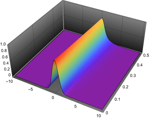
Visualization

lst = Table[{xcol[[i + 1]], tcol[[j + 1]], u[i, j] /. sol}, {i, 0, 
    NN}, {j, 0, M}];

ListPlot3D[Flatten[lst, 1], PlotRange -> All, Mesh -> None, 
 ColorFunction -> "Rainbow", PlotTheme -> "Marketing"]

I have tested this numerical algorithm in a case of Example 1 and 3 as well. It is not so perfect as it mentioned in the paper. Also there are several typos in the equation (5) and (6) in the paper. I try to fix all of them. Code for Example 1:

u0[x_] := 3 c Sech[kap x]^2; ue[x_, t_] := 3 c Sech[kap (x - v t)]^2; 
u1[x_] := 3 c kap v Sech[kap x] Tanh[kap x];
a = -40;
b = 60; NN = 200;
M = 20; alpha = 0; beta = 1; c = 1/10; v = 1 + c; kap = Sqrt[c/(4 v)];
h = (b - a)/NN; xcol = Table[a + h i, {i, 0, NN}];
T = 1; dt = T/M; tcol = Table[dt j, {j, 0, M}];
\[Phi][x_] := (E^(Sqrt[2] x/3) - 2 + E^(-Sqrt[2] x/3))/(2/9);
\[Psi][y_] := Sinh[y];




eqn = Table[(u[n, m + 1] - 
       u[n, m - 1])/(2 \[Psi][dt]) - (u[n + 1, m + 1] - 
       2 u[n, m + 1] + u[n - 1, m + 1] - u[n + 1, m - 1] + 
       2 u[n, m - 1] - u[n - 1, m - 1])/(2 \[Psi][dt] \[Phi][h]) - 
    alpha (u[n + 1, m + 1] - 2 u[n, m + 1] + u[n - 1, m + 1] + 
        u[n + 1, m - 1] - 2 u[n, m - 1] + 
        u[n - 1, m - 1])/(2 \[Phi][
         h]) + (beta + (u[n, m + 1] + u[n, m])/2) (u[n + 1, m + 1] - 
        u[n - 1, m + 1] + u[n + 1, m] - 
        u[n - 1, m])/(4 \[Phi][h]^.5), {n, NN - 1}, {m, M - 1}];
sys = Join[Flatten[Table[eqn[[i, j]] == 0, {i, NN - 1}, {j, M - 1}]], 
   Flatten[
    Table[{u[0, j] == ue[a, tcol[[j]]], 
      u[NN, j] == ue[b, tcol[[j]]]}, {j, 1, M}]], 
   Table[u[i, 0] == u0[xcol[[i + 1]]], {i, 0, NN}], 
   Table[u[i, 1] == u[i, 0] + dt u1[xcol[[i + 1]]], {i, 1, NN - 1}]];
guess = Flatten[Table[{u[i, j], 1/10}, {i, 0, NN}, {j, 0, M}], 1];

sol = FindRoot[sys, guess];


lst = Table[{xcol[[i + 1]], tcol[[j + 1]], u[i, j] /. sol}, {i, 0, 
    NN}, {j, 0, M}];

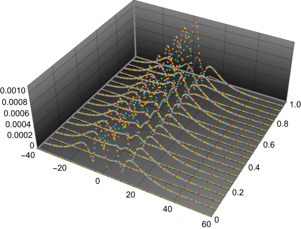
Visualization of error

error = Table[{xcol[[i + 1]], tcol[[j + 1]], 
    Abs[ue[xcol[[i + 1]], tcol[[j + 1]]] - u[i, j] /. sol]}, {i, 0, 
    NN}, {j, 0, M}];

ListPointPlot3D[error, PlotTheme -> "Marketing", PlotRange -> All]

We can compare this result with NDSolve using code @xzczd

With[{u = u[t, x]}, 
 eq = D[u, t] - D[u, x, x, t] - 
    alpha D[u, x, x] + (beta + u) D[u, x] == 0; 
 ic = u == u0[x] /. t -> 0; 
 bc = u == u0[x] /. {{x -> a}, {x -> b}}]; tst2 = 
 Interpolation[Flatten[lst, 1]]; nsol = 
 NDSolveValue[{eq, ic, bc}, u, {t, 0, 1}, {x, a, b}];

With[{t = 1}, 
 Plot[{tst2[x, t], nsol[t, x]}, {x, a, b}, PlotRange -> All]]

With[{t = 1}, 
 Plot[{Abs[tst2[x, t] - ue[x, t]], Abs[nsol[t, x] - ue[x, t]]}, {x, a,
    b}, PlotRange -> All]]