Plotting of probability density on a lattice and studying dynamics

Question

I have a lattice described by a AdjacencyMatrix or Hamiltonian. This matrix has all the information of how each site is connected to another site with what hopping amplitude. For present case, all the hopping amplitudes are 1.
What I want to do:

1. Plotting of probability density $|\Psi_{i,j}|^2$ on this lattice, where $\{i,j\}$ are the lattice sites.
2. Dynamics: On the same lattice, I would be interested if I excite a lattice site at a position $\{i_0,j_0\}$ (initial condition), then how will that excitation or wave propagates in time. Essentially, I am interested in solving the Schrodinger's wave equation. Then looking for the wave solution. For instance, if we excite an eigenstate, then this initial state will remain so even after a long lapse of time. This dynamics is to be seen on the lattice at different discrete times.

My MWE:

(* The Hamiltonian or AdjacencyMatrix of the lattice. Here it is a \
hexagonal lattice *)

hmat = need to be copied from this link

(* The Adjacency graph looks like: hexagonal lattice. *)
  AdjacencyGraph[hmat]

(* Putting coordinates on the hexagonal lattice. *)
  imax = 4; (* the number of rings in the lattice *)

  coords = 
 ArrayFlatten[
  ParallelTable[Table[{i, j}, {j, 12 (i - 1) + 6}], {i, imax}], 1]

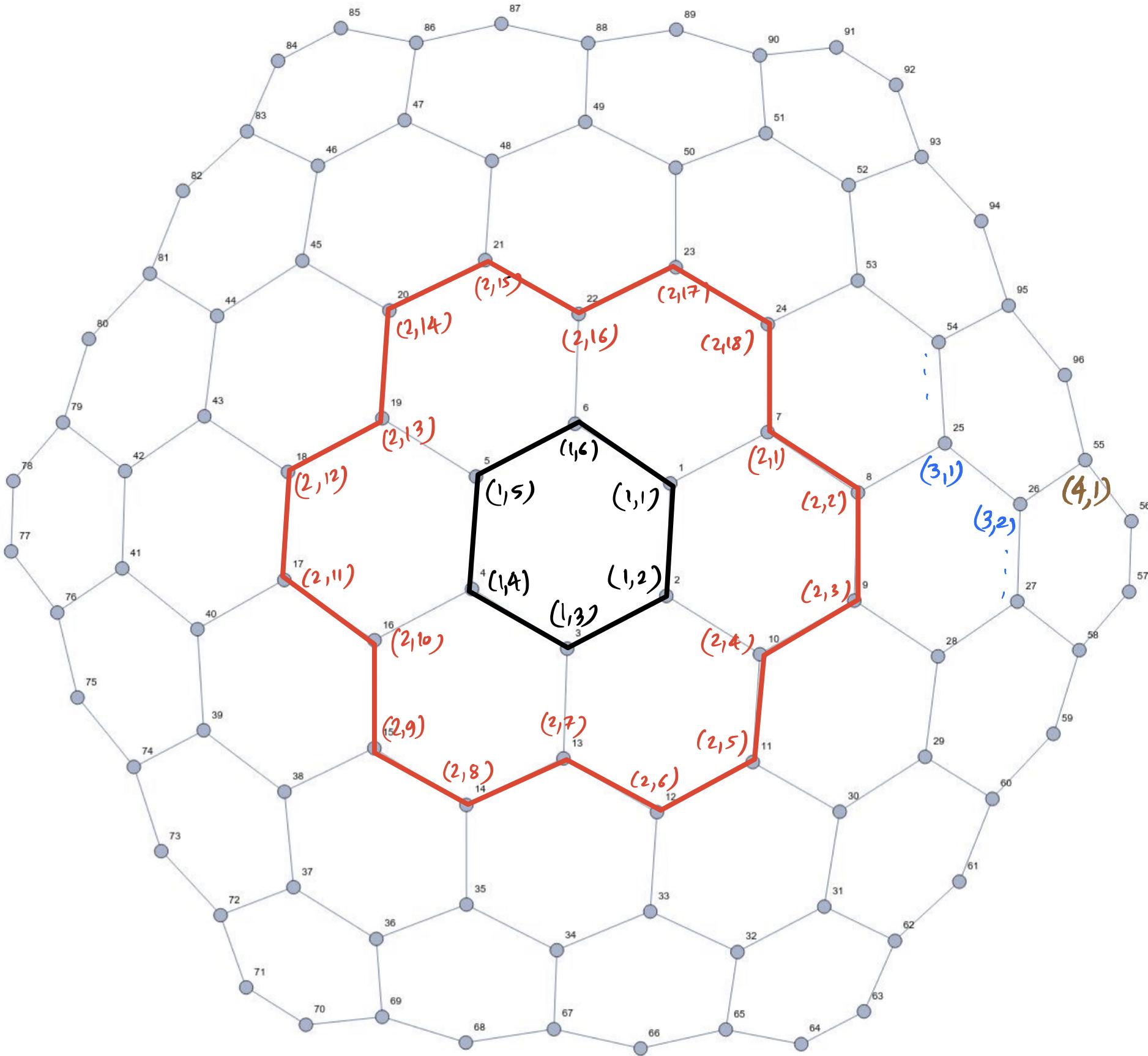
Just to illustrate the above line i.e. coords. The coordinates of the lattice look like (below figure), where the first two rings are highlighted with thick black and red color with proper coordinates going radially. In total, there are four rings imax=4, which can increase or decrease. .

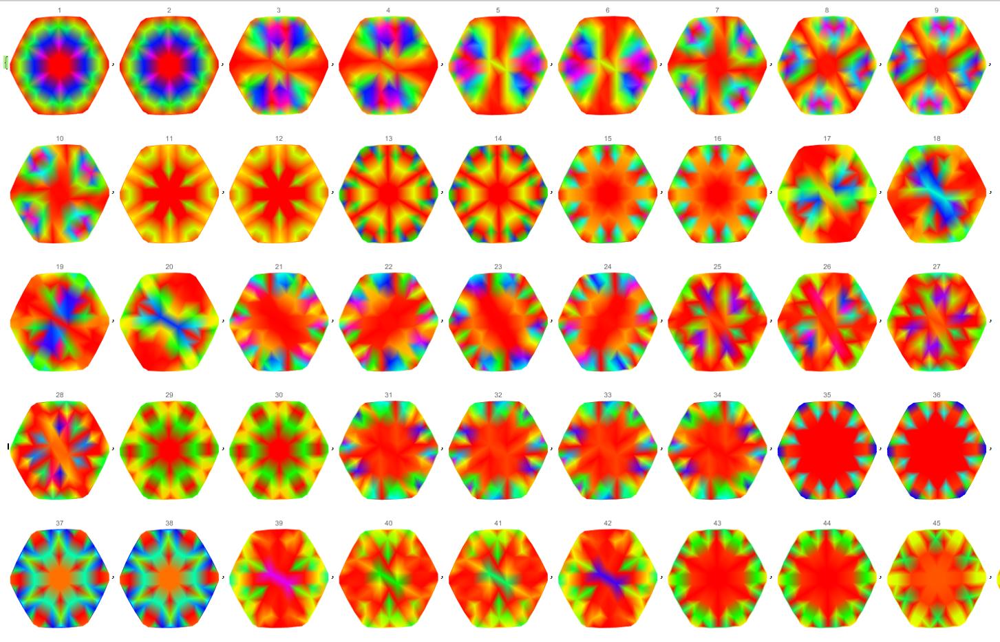
(* Plotting of probability density $|\Psi_{i,j}|^2$ on this lattice *)
vecs = Eigenvectors[hmat // N];

Manipulate[
 ListDensityPlot[
  Table[Append[coords[[i]], Abs[vecs[[n, i]]]^2] // N, {i, 
    Length[vecs[[n]]]}]], {n, 1, Length[vecs], 1}]

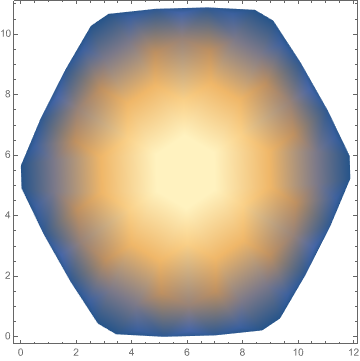
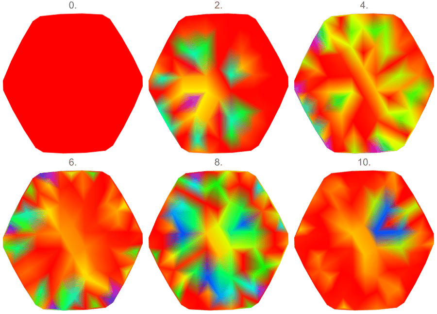
However, the ListDensityPlot comes in a non friendly way, i.e. not in the form of original lattice. Here, x axis is i label and y axis is the j label. It would have been great if it comes in the radial geometry $(r, \theta$). This I can't seem to resolve.

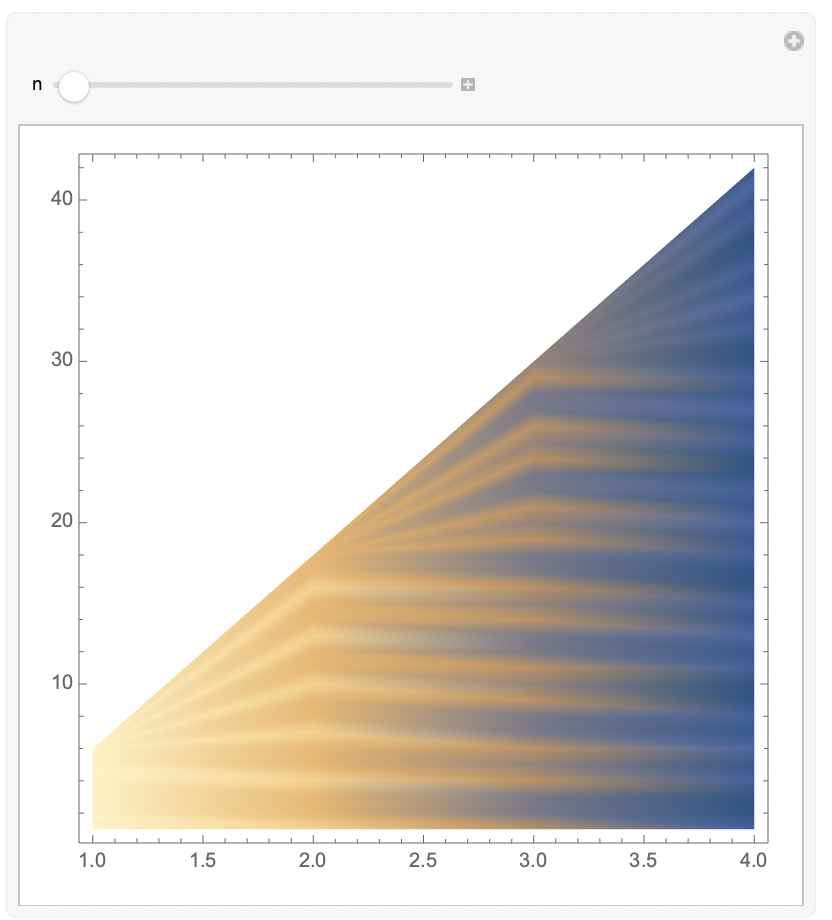
(* The dynamics by solving the Schrodinger equation *)
V[t_] := Table[v[i][t], {i, Length[vecs]}];
sol = NDSolve[{I V'[t] == hmat . V[t], 
    V[0] == Table[KroneckerDelta[i, 10], {i, Length[vecs]}]}, 
   V[t], {t, 0, 100}];

(* The dynamics plot is generated here, but again the plot comes in the same fashion as above not in the usual lattice as shown in the Adjacency graph *)
Manipulate[
 ListDensityPlot[
  Table[N[Append[coords[[i]], Abs[Flatten[V[t] /. sol][[i]]]^2]], {i, 
     Length[vecs]}] /. t -> t1, PlotRange -> {0, 0.05}], {t1, 0, 10}]

Is there a way to resolve this?

Answer 1

Try this:

g = AdjacencyGraph[hmat];
graphCoords = GraphEmbedding[g];
Manipulate[
 ListDensityPlot[
  Table[Append[graphCoords[[i]], Abs[vecs[[n, i]]]^2] // N, {i, 
    Length[vecs[[n]]]}]], {n, 1, Length[vecs], 1}]

Answer 2

There are nice pictures if we use for visualization Hue and Table

g = AdjacencyGraph[hmat];
imax = 4;
 vecs = Eigenvectors[hmat // N];
graphCoords = GraphEmbedding[g];
Table[ListDensityPlot[
  Table[Append[graphCoords[[i]], Abs[vecs[[n, i]]]^2] // N, {i, 
    Length[vecs[[n]]]}], ColorFunction -> Hue, PlotRange -> All, 
  Frame -> False, PlotLabel -> n], {n, 1, Length[vecs], 1}]

Also for dynamics it is better to use animation like this

frames = Table[
   ListDensityPlot[
    Table[N[Append[graphCoords[[i]], 
        Abs[Flatten[V[t] /. sol][[i]]]^2]], {i, Length[vecs]}] /. 
     t -> t1, PlotRange -> All, ColorFunction -> Hue, Frame -> False, 
    ImageSize -> Small, PlotLabel -> t1], {t1, 0, 10, .2}];
ListAnimate[frames]