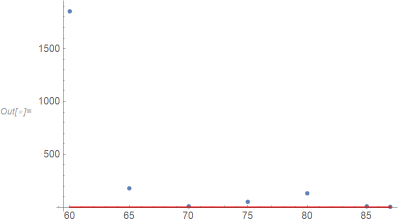
Given that the response and predictor variables are both positive and structure of the model, one of the coefficients (c1 and c2) needs to be negative and the other needs to be positive. Excel's answer at least has that property but I don't see why you say that the Excel answer fits the data relatively well.
data = {{60, 1852.94}, {65, 178.035}, {70, 7.97143}, {75, 48.9479}, {80, 133.561},
  {85, 8.65079}, {87, 1.78915}};

eq = 1/((x*c1)/((Exp[B1/(x - T0)])^0.75)*(1 - Exp[((Tm - x)*c2)/Tm^2])) /.
  {T0 -> 259.246, B1 -> 2595.89, Tm -> 88.2 + 273.15};

excel = {c1 -> -65514626.34, c2 -> 68.4};
Show[ListPlot[data, PlotRange -> All],
 Plot[eq /. excel, {x, 60, 87}, PlotStyle -> Red]]

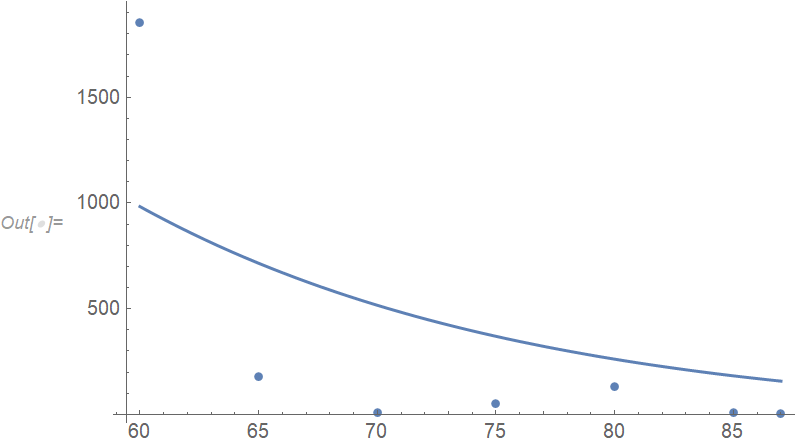
If you start off with estimates of the coefficients with opposite signs, then NonlinearModelFit finds a better fit.
nlm = NonlinearModelFit[data, eq, {{c1, -1}, {c2, 1}}, x, MaxIterations -> 10000];
nlm["BestFitParameters"]
(* {c1 -> 0.000589194, c2 -> -0.000841265} *)
nlm["EstimatedVariance"]^0.5
(* 543.51 *)
Show[ListPlot[data, PlotRange -> All], Plot[nlm[x], {x, 60, 87}]]

Because the estimators of the coefficients given the data and model are nearly perfectly correlated (look at nlm["CorrelationMatrix"]), there is a great deal of numerical instability. In fact, just setting c2 to some arbitrary number and fitting with just c1 gives an even better fit:
nlm = NonlinearModelFit[data, eq /. c2 -> 1, {{c1, -1}}, x, MaxIterations -> 10000];
nlm["BestFitParameters"]
(* {c1 -> -4.95197*10^-7} *)
nlm["EstimatedVariance"]^0.5
(* 496.162 *)
Show[ListPlot[data, PlotRange -> All], Plot[nlm[x], {x, 60, 87}]]

But all fits are horrible. To paraphrase Bullwinkle the Moose: "You need a better model."


Show[{ ListPlot[data], Plot[(E^(2595.89/(-259.246 + x)))^0.75/(c1 (1 - E^(5.092118394960718*^-6 c2 (443.15 - x))) x) /. {c1 ->313634, c2 -> -8434.47}, {x, First[data][[1]], Last[data][[1]]}, PlotRange -> All]. It shows that the values of c1 and c2 you obtained from excel yield a very bad fit, if any. $\endgroup$