If I have the following data:
Tgexpandlit={{57.8505, 1.36339}, {58.1254, 1.0671}, {58.7645, 0.646116}, {59.221,
  0.349873}, {60.6788, -0.273668}, {62.7712, -0.803456}, {64.3186, \
-1.28659}, {64.3186, -1.28659}, {66.5927, -1.83193}, {68.7745, \
-2.20572}, {71.0471, -2.57948}, {72.7748, -2.92218}, {74.3203, \
-3.20255}, {76.138, -3.45164}, {78.5006, -3.74739}, {80.2275, \
-3.99651}, {81.4994, -4.12096}, {82.6805, -4.24544}, {83.4074, \
-4.32324}, {84.1346, -4.44783}, {85.1342, -4.57236}, {86.3147, \
-4.61885}, {87.1328, -4.75901}, {88.2229, -4.85232}, {88.859, \
-4.93014}, {90.04, -5.03902}, {91.4019, -5.06986}, {92.2198, \
-5.17884}, {93.4007, -5.28772}, {93.3998, -5.17853}, {94.4905, \
-5.34983}, {96.4889, -5.50529}, {97.3069, -5.62986}, {99.1234, \
-5.75417}, {99.2131, -5.62936}, {99.8498, -5.76958}, {101.848, \
-5.87825}, {101.847, -5.83145}, {102.575, -5.95605}, {103.936, \
-5.98689}, {105.389, -6.0489}, {53.05, 1.02729}, {54.3782,
  0.553702}, {54.2158,
  0.0303926}, {56.9221, -0.439578}, {59.0303, -0.956926}, {62.3764, \
-1.42534}, {66.8545, -1.9367}, {69.3497, -2.40747}, {70.7512, \
-2.70496}, {71.6037, -2.92466}, {51.2734, 1.02255}, {52.1209,
  0.547695}, {52.3608,
  0.0254565}, {55.4547, -0.443448}, {56.8651, -0.962607}, {59.8218, \
-1.43198}, {65.7229, -1.9396}, {69.0066, -2.40835}, {70.6466, \
-2.70522}, {71.5932, -2.92468}, {54.5032, 1.03115}, {54.9453,
  0.555205}, {56.6674,
  0.0368729}, {57.758, -0.437381}, {60.2665, -0.9537}, {62.7824, \
-1.42429}, {66.8842, -1.93663}, {69.7442, -2.40648}, {71.3554, \
-2.70343}, {72.963, -2.92124}, {53.05, 1.02729}, {54.4775,
  0.553965}, {54.7589,
  0.0318322}, {58.2357, -0.436128}, {60.1001, -0.954134}, {63.2519, \
-1.42308}, {66.8886, -1.93662}, {69.3662, -2.40743}, {70.8179, \
-2.70479}, {71.7396, -2.92431}, {51.2734, 1.02255}, {52.2206,
  0.547961}, {52.8968,
  0.0268856}, {56.701, -0.44016}, {57.9147, -0.959849}, {60.6854, \
-1.42973}, {65.7529, -1.93952}, {69.0215, -2.40831}, {70.7068, \
-2.70507}, {71.7159, -2.92437}, {54.5032, 1.03115}, {55.0455,
  0.55547}, {57.1738,
  0.0382057}, {59.0075, -0.434107}, {61.2621, -0.95111}, {63.6165, \
-1.42214}, {66.9159, -1.93655}, {69.7599, -2.40644}, {71.4196, \
-2.70327}, {73.0906, -2.92092}, {51.139, 2.32322}, {52.2163,
  1.80322}, {53.1749, 1.32866}, {53.6977, 1.02902}, {54.1641,
  0.808406}, {54.7846, 0.554779}, {55.0134, 0.333536}, {50.6163,
  2.32182}, {52.0102, 1.80267}, {52.6447, 1.32724}, {53.6972,
  1.02902}, {54.1492, 0.808367}, {54.1878, 0.553197}, {54.8392,
  0.333075}, {52.6762, 2.32733}, {53.7473, 1.8073}, {54.0918,
  1.33109}, {55.3849, 1.03349}, {55.5279, 0.812018}, {55.6434,
  0.557051}, {55.9373, 0.335978}}
and I am fitting it to a function such as:
   Eappitz = 99.925; q0 = 10/60; Tg0itz = 54.26 + 273.15; Aitz =
 Log10[(Tg0itz^2)/(q0*Eappitz*1000)];

(nlm = NonlinearModelFit[
    Tgexpandlit, {((-C11 (T + 273.15 - Tg0itz))/(C22 + (T + 273.15 -
            Tg0itz))) + Aitz}, {C11, C22}, T]) // Normal

nlm["BestFitParameters"]

C1itz = C11 /. nlm["BestFitParameters"](*7.76*);
C2itz = C22 /. nlm["BestFitParameters"](*19.22*);


fitz[T_] := ((-C1itz (T + 273.15 - Tg0itz))/(C2itz + (T + 273.15 -
        Tg0itz))) + Aitz
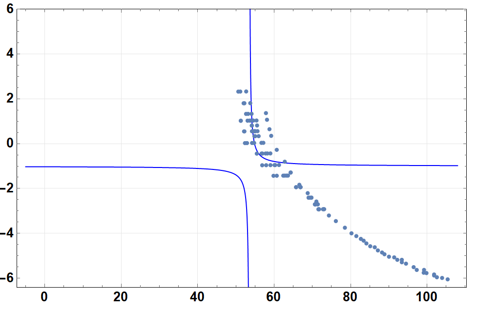
I get a very bad fit such as the following:
Show[Plot[fitz[T], {T, -5, 108}, Frame -> True, FrameStyle -> 16,
  Axes -> False, GridLines -> Automatic,
  GridLinesStyle -> Lighter[Gray, .8],
  FrameTicks -> {Automatic, Automatic}, ImageSize -> Large,
  LabelStyle -> {Black, Bold, 14}, PlotStyle -> Blue,
  PlotRange -> {All, {-6.4, 6}}]

 , ListPlot[Tgexpandlit]]
Which gives:
However, If I only use the first portion of the same data such as:
Tgexpandlit={{57.8505, 1.36339}, {58.1254, 1.0671}, {58.7645, 0.646116}, {59.221,
  0.349873}, {60.6788, -0.273668}, {62.7712, -0.803456}, {64.3186, \
-1.28659}, {64.3186, -1.28659}, {66.5927, -1.83193}, {68.7745, \
-2.20572}, {71.0471, -2.57948}, {72.7748, -2.92218}, {74.3203, \
-3.20255}, {76.138, -3.45164}, {78.5006, -3.74739}, {80.2275, \
-3.99651}, {81.4994, -4.12096}, {82.6805, -4.24544}, {83.4074, \
-4.32324}, {84.1346, -4.44783}, {85.1342, -4.57236}, {86.3147, \
-4.61885}, {87.1328, -4.75901}, {88.2229, -4.85232}, {88.859, \
-4.93014}, {90.04, -5.03902}, {91.4019, -5.06986}, {92.2198, \
-5.17884}, {93.4007, -5.28772}, {93.3998, -5.17853}, {94.4905, \
-5.34983}, {96.4889, -5.50529}, {97.3069, -5.62986}, {99.1234, \
-5.75417}, {99.2131, -5.62936}, {99.8498, -5.76958}, {101.848, \
-5.87825}, {101.847, -5.83145}, {102.575, -5.95605}, {103.936, \
-5.98689}, {105.389, -6.0489}}
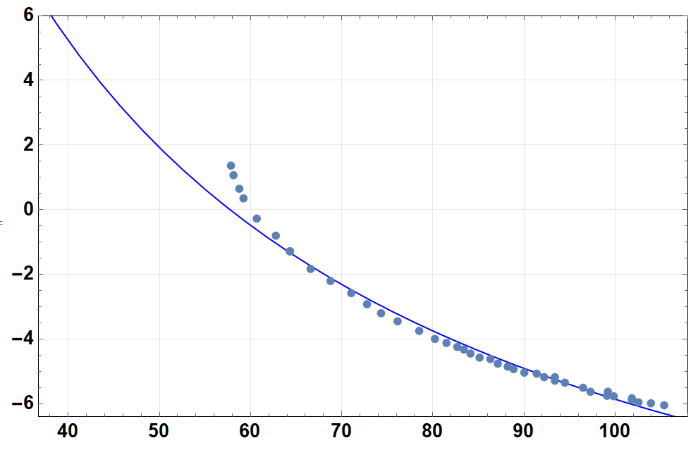
I now get a great fit like:
Question:
- Why cannot use all the data or how can I arrange the data so that all the data can be used to get the fit? (as opposed to only part of the same data)


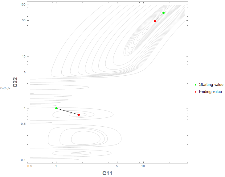
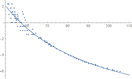
{{C11, 17}, {C22, 70}}as the parameter specification in yourNonlinearModelFit. The importance of providing good starting values for parameters in fitting cannot be overstated. $\endgroup$