4
$\begingroup$

A simple 3-dimensional ODE system is given:

$F=\begin{cases} \dot{x}=g+g_{U_{rep}} \\ \dot{g}=-g+\frac{df}{dx} \\ \dot{h}=-h+\frac{d^2f}{d^2x} \end{cases} $

Task: Make the variable $g$ move so that it bounces off the barrier $\psi=\delta +\frac{2-\delta }{t T+1}$

where:

$x,g,h$ - state-space variables

$f=-x^2$

$T, \delta$ - positive numbers;

$g_{U_{rep}}=F_{APF}(g)$ - repulsive barrier;

$t$ - time;

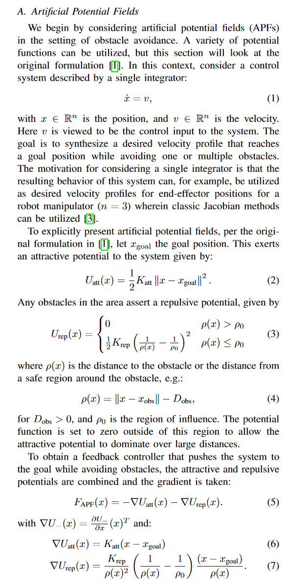
I want to use artificial potential barriers that allow ODE variable to avoid obstacles. They are constructed as follows. https://authors.library.caltech.edu/106548/1/2010.09819.pdf

enter image description here

There is my code:

Clear["Derivative"]

ClearAll["Global`*"]

pars = {xs = -1, xe = 1/2, T = 1/2, \[Delta] = 0.35};

f = -(x[t])^2

(***)

\[Psi]obs = (1 - \[Delta])/(T t + 1) + \[Delta]

krep = 1; dobs = 0.25; \[Rho]0 = 0.25;

\[Rho] = Norm[{G[t] - \[Psi]obs}, 2] - dobs

gUrep = Piecewise[{{krep/\[Rho]^2 (1/\[Rho] - 1/\[Rho]0) G[
       t]/\[Rho], \[Rho] <= \[Rho]0}, {0, \[Rho] > \[Rho]0}}]

Plot[{\[Psi]obs}, {t, 0, 100}, PlotRange -> Full]

(***)

sys = NDSolve[{x'[t] == G[t] + gUrep, G'[t] + G[t] == D[f, x[t]], 
   H'[t] + H[t] == D[f, {x[t], 2}], x[0] == xs, G[0] == 0.5, 
   H[0] == 0}, {x, G, H}, {t, 0, 500}, 
  Method -> {"DiscontinuityProcessing" -> False}]

Plot[{Evaluate[x[t] /. sys], xe}, {t, 0, 100}, PlotRange -> Full, 
 PlotPoints -> 200]

Plot[{Evaluate[G[t] /. sys], \[Psi]obs}, {t, 0, 100}, 
 PlotRange -> Full, PlotPoints -> 200]

Plot[{Evaluate[gUrep /. sys]}, {t, 0, 4}, PlotRange -> Full, 
 PlotPoints -> 200]

I want to visualize the movement of a system in a steady-state with barriers and also how a variable pushes against these barriers in this system. I don't know how to correctly express this: vector space visualization, phase-space visualization, etc.

We may need commands: ParametricPlot3D and ParametricPlot

$\endgroup$
4
  • 1
    $\begingroup$ In your example system not approaches barrier. Do you mean parametric research to find out some parameters of gUrep first? $\endgroup$ Commented May 21, 2021 at 15:37
  • $\begingroup$ @AlexTrounev it is a repulsive barrier that the variable should not approach. in other words, the trajectory that the variable should not jump over. $\endgroup$
    – ayr
    Commented May 21, 2021 at 20:07
  • $\begingroup$ With your parametrs gUrep=0 for `{t,0,500}'. That is the reason to define this function? $\endgroup$ Commented May 21, 2021 at 20:18
  • $\begingroup$ @AlexTrounev $\delta +\frac{1-\delta }{t T+1}$; $G(0)=0$ Alex, I changed $\psi$ to something else, and also changed the initial condition for $G$. Now the barrier has a response. I updated the new version of the code. $\endgroup$
    – ayr
    Commented May 22, 2021 at 4:18

1 Answer 1

4
$\begingroup$

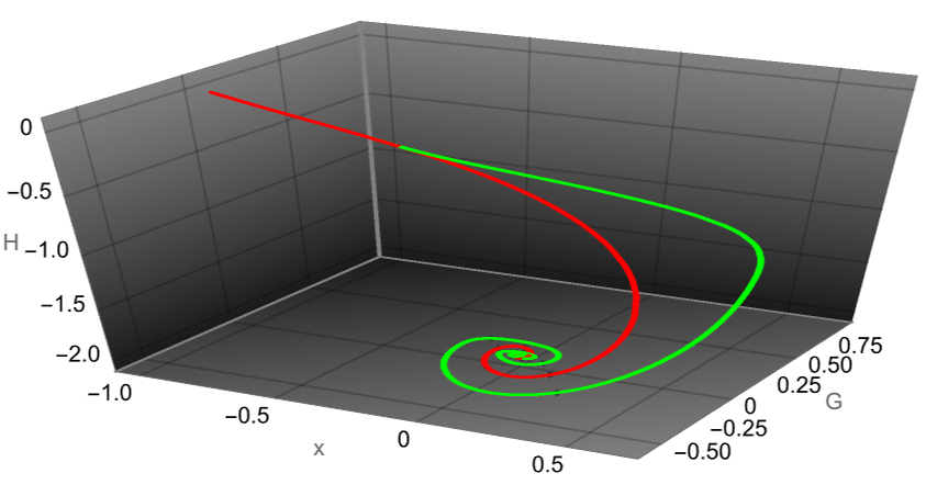
We can compare scenario with (green line) and without (red line) barrier as follows

Clear["Derivative"]

ClearAll["Global`*"]

pars = {xs = -1, xe = 1/2, T = 1, \[Delta] = .35};

f = -(x[t])^2;

(***)

\[Psi]obs = (2 - \[Delta])/(T t + 1) + \[Delta];

krep = 1; dobs = 0.05; \[Rho]0 = 0.75;

\[Rho] = Norm[{G[t] - \[Psi]obs}, 2] - dobs;

gUrep = Piecewise[{{krep/\[Rho]^2 (1/\[Rho] - 1/\[Rho]0) G[
        t]/\[Rho], \[Rho] <= \[Rho]0}, {0, \[Rho] > \[Rho]0}}];

Plot[{\[Psi]obs}, {t, 0, 100}, PlotRange -> Full]

(***)

sys = NDSolve[{x'[t] == G[t] + gUrep, G'[t] + G[t] == D[f, x[t]], 
    H'[t] + H[t] == D[f, {x[t], 2}], x[0] == xs, G[0] == 0, 
    H[0] == 0}, {x, G, H}, {t, 0, 500}, 
   Method -> {"DiscontinuityProcessing" -> False}];


sys0 = NDSolve[{x'[t] == G[t] + 0 gUrep, G'[t] + G[t] == D[f, x[t]], 
    H'[t] + H[t] == D[f, {x[t], 2}], x[0] == xs, G[0] == 0, 
    H[0] == 0}, {x, G, H}, {t, 0, 500}, 
   Method -> {"DiscontinuityProcessing" -> False}];

ParametricPlot3D[{Evaluate[{x[t], G[t], H[t]} /. sys], 
  Evaluate[{x[t], G[t], H[t]} /. sys0]}, {t, 0, 50}, 
 PlotStyle -> {Green, Red}, PlotRange -> All, AspectRatio -> 1/2, 
 Boxed -> False, AxesLabel -> {"x", "G", "H"}, ImageSize -> 400, 
 PlotTheme -> "Marketing"] 

Figure 1

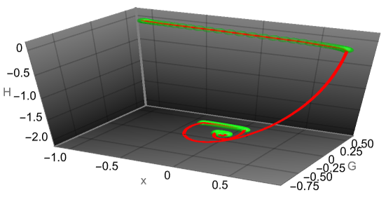
We can show part of trajectory where $\rho < \rho_0$ as follows

pars = {xs = -1, xe = 1/2, T = 1/2, \[Delta] = 0.35};

f = -(x[t])^2;

(***)

\[Psi]obs = (1 - \[Delta])/(T t + 1) + \[Delta];

krep = 1; dobs = 0.25; \[Rho]0 = 0.25;

\[Rho] = Norm[{G[t] - \[Psi]obs}, 2] - dobs;

gUrep = Piecewise[{{krep/\[Rho]^2 (1/\[Rho] - 1/\[Rho]0) G[
        t]/\[Rho], \[Rho] <= \[Rho]0}, {0., \[Rho] > \[Rho]0}}];

Plot[{\[Psi]obs}, {t, 0, 100}, PlotRange -> Full]

(***)

sys = NDSolve[{x'[t] == G[t] + gUrep, G'[t] + G[t] == D[f, x[t]], 
    H'[t] + H[t] == D[f, {x[t], 2}], x[0] == xs, G[0] == 0.5, 
    H[0] == 0}, {x, G, H}, {t, 0, 500}, 
   Method -> {"DiscontinuityProcessing" -> False}];

sys0 = NDSolve[{x'[t] == G[t] + 0 gUrep, G'[t] + G[t] == D[f, x[t]], 
    H'[t] + H[t] == D[f, {x[t], 2}], x[0] == xs, G[0] == 0.5, 
    H[0] == 0}, {x, G, H}, {t, 0, 500}, 
   Method -> {"DiscontinuityProcessing" -> False}];
tms = Table[
   If[First[Evaluate[(\[Rho] - \[Rho]0) /. sys]] < 0, t, Nothing], {t,
     0, 10, .002}];

obst = Graphics3D[
  Table[{Green, Opacity[.25], 
    Sphere[Evaluate[{x[t], G[t], H[t]} /. sys], .05]}, {t, tms}]];

Show[ParametricPlot3D[{Evaluate[{x[t], G[t], H[t]} /. sys]}, {t, 0, 
   50}, PlotStyle -> {Green, Red}, PlotRange -> All, 
  AspectRatio -> 1/2, Boxed -> False, AxesLabel -> {"x", "G", "H"}, 
  ImageSize -> 400, PlotTheme -> "Marketing"], obst]

Figure 2

$\endgroup$
4
  • $\begingroup$ can we add another one to this figure, but replace $g$ to \psi ? $\endgroup$
    – ayr
    Commented May 21, 2021 at 20:09
  • $\begingroup$ Do you mean replace G with \[Psi]obs? Then what is the sense of this plot? $\endgroup$ Commented May 21, 2021 at 20:21
  • $\begingroup$ Yes. The meaning of the graph is as follows: $\psi$ sets the trajectory to which the variable $G$ cannot go. I would like to clearly see how this happens. In the articles where I got this from, they build obstacle avoidance on the plane. I would like to get something similar. $\endgroup$
    – ayr
    Commented May 22, 2021 at 4:27
  • $\begingroup$ In such a setting, there really is not much sense, but I want to somehow visualize the work of the system, how its phase space changes (when I add a barrier) and how the system moves in this space. But I don't know of any other form of visualization of this. For example: downloads.hindawi.com/journals/mpe/2020/6523158.pdf [p. 11-16] $\endgroup$
    – ayr
    Commented May 22, 2021 at 4:29

Your Answer

By clicking “Post Your Answer”, you agree to our terms of service and acknowledge you have read our privacy policy.

Not the answer you're looking for? Browse other questions tagged or ask your own question.