3
$\begingroup$

Given:

$\begin{cases} \dot{x}=-x^2+\frac{1}{y+1}+1 \\ \dot{y}=1 \end{cases}$

I am trying to linearize the system in the classical way, using the Jacobi matrix.

asys = AffineStateSpaceModel[{x'[t] == -x[t]^2 + 1/(y[t] + 1) + u[t], 
    y'[t] == 1}, {{x[t]}, {y[t]}}, {u[t]}, {x[t]}, t] 

or2 = OutputResponse[asys, 1, {t, 0, 20}];

Plot[{or2}, {t, 0, 20}, PlotRange -> Full];

 eq = N[Normal[Solve[{-x[t] + 1/(y[t] + 1) + 1, 1} == {0, 0}, {x[t], y[s]}, Reals]]];

Stuck at the last stage, where the equilibrium points of the vector field are sought. Stuck because the right side of second equation is $1$ and it can't be $0$anywhere. How to get around this obstacle?

I would be grateful for help.

$\endgroup$
5
  • $\begingroup$ As you noticed, there is no equilibrium of this system because $y$ keeps increasing. Since $dy/dt$ is independent of $x$ you can see that $y(t)=y(0)+t$. This makes the $1/(y+1)$ term in $dx/dt$ go to zero as $t\to\infty$, so the long-term behavior of $x$ can be found by studying $dx/dt=1-x^2$. $\endgroup$
    – Chris K
    Commented Aug 10, 2021 at 13:07
  • $\begingroup$ @ChrisK I agree, In this form, the system does not lend itself to linearization, Because it has no equilibrium points. But, maybe the original $\dot{x}=-x^2+\frac{1}{t+1}+1$ can be linearized? A comment was left there, it is not an option, because non-autonomy can be more complex and some more or less universal approach is needed. $\endgroup$
    – ayr
    Commented Aug 10, 2021 at 13:17
  • $\begingroup$ Yes, you can linearize around the trajectory of the nonlinear system (see math.stackexchange.com/questions/1254711/… for example). Let $z(t)$ be the deviation from the nominal trajectory $x(t)$ that you get from solving $dx/dt$. Then $dz/dt=(d\dot x/dx)z=-2xz$. $\endgroup$
    – Chris K
    Commented Aug 10, 2021 at 16:00
  • $\begingroup$ @ChrisK Could you provide an example in Mathematical? $\endgroup$
    – ayr
    Commented Aug 10, 2021 at 19:15
  • $\begingroup$ Sure (note I changed notation from $z$ to $\delta x$) $\endgroup$
    – Chris K
    Commented Aug 10, 2021 at 20:08

2 Answers 2

2
$\begingroup$

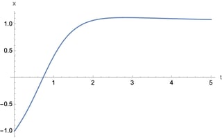
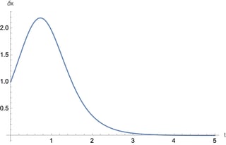
The following solves the nonlinear equation $dx/dt$ along with the linearized variational equation $d(\delta x)/dt$:

f[x_] := -x^2 + 1/(t + 1) + 1;
tmax = 5;
sol = NDSolve[{
  x'[t] == f[x[t]], δx'[t] == f'[x[t]]*δx[t],
  x[0] == -1, δx[0] == 1}, {x, δx}, {t, 0, tmax}][[1]];

Plot[Evaluate[x[t] /. sol], {t, 0, tmax}, PlotRange -> All]
Plot[Evaluate[δx[t] /. sol], {t, 0, tmax}, PlotRange -> All]

enter image description here

enter image description here

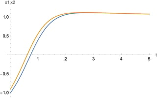
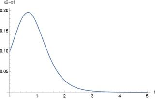
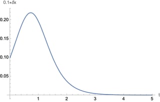
The bottom plot shows that nearby trajectories initially diverge, but eventually come back together again ($\delta x\to0$ as $t\to\infty$). To see how that works, we can solve two copies of the nonlinear system with (relatively) close initial conditions, plot their difference, and compare against the variational result:

sol2 = NDSolve[{
  x'[t] == f[x[t]], x2'[t] == f[x2[t]],
  x[0] == -1, x2[0] == -1 + 0.1}, {x, x2}, {t, 0, tmax}][[1]];

Plot[Evaluate[{x[t], x2[t]} /. sol2], {t, 0, tmax}, PlotRange -> All]
Plot[Evaluate[x2[t] - x[t] /. sol2], {t, 0, tmax}, PlotRange -> All]
Plot[Evaluate[0.1*δx[t] /. sol], {t, 0, tmax}, PlotRange -> All]

enter image description here

enter image description here

enter image description here

Pretty close (not perfect since the initial perturbation of 0.1 isn't too small).

$\endgroup$
5
  • $\begingroup$ Thank you for your answer! Here's what I noticed. Numerical analysis shows that the system passes from the initial state to the equilibrium point along a very smooth trajectory. But the system of equations that is used in numerical analysis cannot be called linear. Tell me, is it possible to obtain an equivalent linear system in such a way as if we used Jacobi matrices, i.e. differential equations of the form $\dot{z}=Jz$? $\endgroup$
    – ayr
    Commented Aug 11, 2021 at 2:33
  • 1
    $\begingroup$ In my solution the equation for δx'[t] is indeed in the same form you requested (it's a one-dimensional system, so no matrices needed). When we linearize around an equilibrium as often done, the "reference solution" is just a point, so the equation for the perturbation is unforced. Here we have to linearize around a trajectory, not a point, which we need to solve numerically. The same idea is used in calculating Floquet and Lyapunov exponents. Check out these notes for a nice overview. $\endgroup$
    – Chris K
    Commented Aug 11, 2021 at 12:23
  • $\begingroup$ It became more or less clear, but not completely. In general, referring to these tools, I wanted to reduce the nonlinear ODE system to a linear one in order to be able, for example, to work with transfer functions. This is necessary to describe transient processes analytically. Yes, some of the properties will be lost, but a rough estimate will be enough. $\endgroup$
    – ayr
    Commented Aug 11, 2021 at 13:18
  • 1
    $\begingroup$ Sorry, I've mostly forgotten about transfer functions since college. Maybe someone else could advise. $\endgroup$
    – Chris K
    Commented Aug 11, 2021 at 14:43
  • $\begingroup$ Reduction of nonlinear systems is a very interesting topic. The more versatile the apparatus is, the better, but so far there is no such thing. $\endgroup$
    – ayr
    Commented Aug 11, 2021 at 16:56
4
$\begingroup$

Since $y(t)$ is $t$, we can find an equilibrium value for $u$ as a function of $t$ and $xt$ (the value of $x(t)$ at time $t$).

ueql = u[t] /. Solve[-x[t]^2 + 1/(y[t] + 1) + u[t] == 0, u[t]][[1]] /. 
       {x[t] -> xt, y[t] -> t}

$\frac{t \text{xt}^2+\text{xt}^2-1}{t+1}$

Now we can assemble a nonlinear state-space model.

nsys = NonlinearStateSpaceModel[{x'[t] == -x[t]^2 + 1/(t + 1) + u[t]}, 
       {{x[t], xt}}, {{u[t], ueql}}, {x[t]}, t]

enter image description here

When $x(t)$ is $xt$ and $u(t)$ is $ueql$, the r.h.s of the above NonlinearStateSpaceModel is $0$.

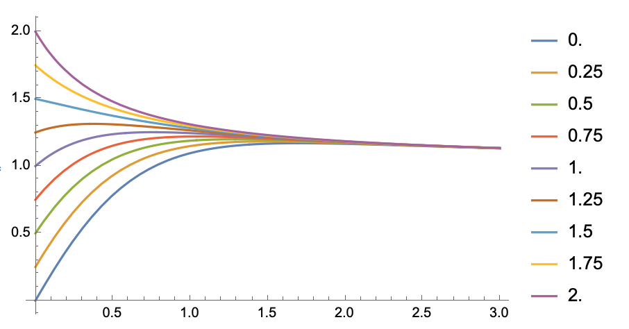
If the input it set to $1$, we get the following responses for various $xt$ values.

Table[OutputResponse[nsys /. xt -> xtVal, 1, {t, 0, 5}][[1]], {xtVal, 0, 2, 0.25}];
Plot[%, {t, 0, 3}, PlotRange -> All, PlotLegends -> Table[xtVal, {xtVal, 0, 2, 0.25}]]

enter image description here

$\endgroup$
1
  • $\begingroup$ Thank you for your answer! I did not quite understand what the linearization is, if the initial system is used in the numerical analysis, and the stable position of the input signal is not used in any way. Could you clarify this ? In general, I expected to get a result similar to linearization using the Jacobi matrix. Is it possible? $\endgroup$
    – ayr
    Commented Aug 11, 2021 at 2:30

Your Answer

By clicking “Post Your Answer”, you agree to our terms of service and acknowledge you have read our privacy policy.

Not the answer you're looking for? Browse other questions tagged or ask your own question.