Numerical Simulation of a Damped, Driven Nonlinear Wave System with Spatially Extended Initial Conditions

Question

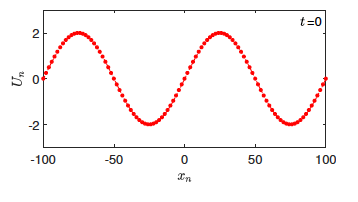
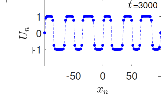
I am working on a project that requires creating a specific type of graph, but I am having trouble writing the correct code. The graph should look similar to the one I have attached below.

Could someone please provide guidance on how to correctly create this type of graph? Any help with the code or tips would be greatly appreciated!

Thank you in advance for your assistance!

THE PROJECT

The study of the dynamics of the discrete Klein - Gordon equation (DKG) with friction is given by the equation : $$\ddot {U} _n - k (U_ {n + 1} - 2 U_n + U_ {n - 1}) + \delta\dot {U} \ _n + W' (U_n) = 0;\quad\beta > 0, \delta > 0 \ \ (1)$$

In the above equation, W describes the potential function:$W (U_n) = -\frac {w_d^2} {2} U_n^2 + \frac {\beta w_d^4} {4} U_n^4$

to which every coupled unit $U_n$ adheres. In Eq. (1), the variable $U_n(t)$ is the unknown displacement of the oscillator occupying the n-th position of the lattice, and $k=h^{-2}$ is the discretization parameter. We denote by h the distance between the oscillators of the lattice. The chain (DKG) contains linear damping with a damping coefficient $\delta>0$, while $\beta$ is the coefficient of the nonlinear cubic term.

For the DKG chain (1), we will consider the problem of initial-boundary values, with initial conditions

$$U_n(0) = U_ {n,0} \quad \text{and} \quad \dot{U}_n(0) = U_ {n,1} \in \ \mathbb{R}^{K+2},\ \ (2)$$

and Dirichlet boundary conditions at the boundary points $x_0 = -L/2$ and $x_{K+1} = L/2$, that is,

$$U_0 = U_{K+1} = 0, \quad t \geq 0.\ \ (3)$$

Therefore, when necessary, we will use the short notation $\Delta_d$ for the one-dimensional discrete Laplacian

$$\{\Delta_d U\}_{n \in \mathbb{Z}} = U_{n+1} - 2U_n + U_{n-1} \ \ (4)$$

Now we want to investigate numerically the dynamics of the system (1)-(2)-(3). Our first aim is to conduct a numerical study of the property of Dynamic Stability of the system, which directly depends on the existence and linear stability of the branches of equilibrium points.

For the discussion of numerical results, it is also important to emphasize the role of the parameter $\omega_d^2$. By changing the time variable $t \rightarrow \frac{t}{h}$ , we rewrite Eq. (1) in the form

\begin{equation}\ddot{U}_n - \Delta_d U + \hat{\delta} \dot{U}_n = \Omega_d^2 (U_n - \beta U_n^3), \quad t > 0, \quad \Omega_d^2 = h^2 \omega_d^2, \quad \hat{\delta} = h \delta\end{equation}. We consider spatially extended initial conditions of the form:$$ U_n(0) = U_{n,0} = a \sin \left( \frac{j \pi h n}{L} \right), \quad j = 1, \ldots, K $$ where $ h = \frac{L}{K+1} $ is the distance of the grid and $ a > 0$ is the amplitude of the initial condition

We also assume zero initial velocity: $\dot{U}_n(0) = U_{n,1} = 0 $. I want to create the following graphs for $a=2, K=99,L=200,\beta=1, \delta=0.05$ and $\omega_d^2=1$

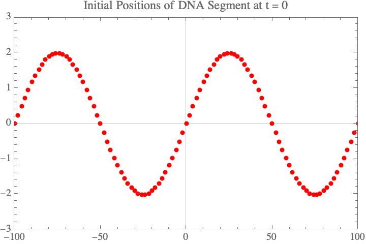
For the first plot, I created the following code!

(*Parameters*)
a = 2;(*Amplitude of the initial condition*)
j = 2; (*Mode number*)
l = 200; (*Length of the system*)
k = 99; (*number of spatial points*)

(*spatial grid*)
h = l/(k + 1);
n = Range[-l/2, l/2, h]; (*spatial points*)

(*compute u_n(0) for each n*)
uN0 = a*Sin[(j*Pi*h*n)/l];


(*Plotting the initial positions*)ListPlot[Transpose[{n, uN0}], PlotStyle -> {Red, PointSize[Medium]}, 
AxesLabel -> {"x_n", "u_n"}, 
PlotLabel -> "Initial Positions of DNA Segment at t = 0", 
PlotTheme -> "Scientific", PlotRange -> {{-l/2, l/2}, {-3, 3}}]

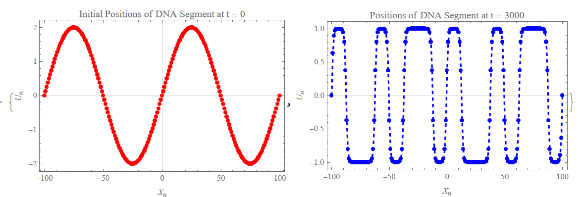
I don't know how to create a proper code to create the blue graph for my problem

L = 200;  (*Number of base pairs,representing a segment of DNA*)
kappa = 1;    (*discretization parameter*)
omegaD = 1;   (*characteristic frequency*)
beta = 1;    (*Nonlinearity parameter*)
delta = 0.05;   (*Damping coefficient*)
j = 2; (*Mode number*)

k = 99; (*number of spatial points*)
(*spatial grid*)h = L/(k + 1);
nsp = Subdivide[-L/2, L/2, k + 1];(*Spatial points*)

(*Scaled parameters*)omegaD2 = (h^2)*omegaD^2;
deltaHat = h*delta;
a = 2;(*Amplitude of the initial condition*)

(*Sinusoidal initial perturbations to simulate thermal fluctuations*)
initialPositions = Table[x[n][0] == a*Sin[j*Pi*n*h/L], {n, 1, L}];
initialVelocities = 
 Table[x[n]'[0] == 0, {n, 1, L}];  (*Assuming initial rest state*)

(*Boundary Conditions*)
boundaryConditions = {x[1][t] == 0, x[L][t] == 0};

(*Equations*)
equations = 
 Table[x[n]''[t] - kappa (x[n + 1][t] - 2 x[n][t] + x[n - 1][t]) + 
    deltaHat x[n]'[t] + omegaD2^2 (x[n][t] - beta x[n][t]^3) == 
   0, {n, 1, L}];

(*Solve Numerically*)
solution = 
 NDSolveValue[{equations, initialPositions, initialVelocities, 
   boundaryConditions}, Table[x[n], {n, 1, L}], {t, 0, 3000}, 
  Method -> {"IndexReduction" -> Automatic} ];(*Visualization*)

Plot[Evaluate[Table[solution[[n]][t], {n, 1, L}]], {t, 0, 3000}, 
PlotLegends -> Table[StringJoin["Base ", ToString[n]], {n, 1, L}], 
PlotRange -> All]
'''

Answer 1

We can play with parameters to make same plot, but with current data we have

(*parameters*)a = 2;(*Amplitude of the initial condition*)
j = 2; (*Mode number*)
L = 200; (*Length of the system*)

omegad = 1; (*characteristic frequency*)
beta = 1;(*Nonlinearity parameter*)

(*damping coefficient*)
delta = 0.05;

(*spatial grid*)
h = 1;
grid = Range[-L/2, L/2, h];(*Spatial points*)
k = Length[grid]; (*number of spatial points*)
(*discretization parameter*)
(*Scaled parameters*)
omegad2 = (h^2)*omegad^2;
deltaHat = h*delta;

tmax = 3000; (*Maximum time*)


var = Table[u[i][t], {i, k}]; eqs = 
 Table[u[i]''[t] - (u[i + 1][t] + u[i - 1][t] - 2  u[i][t]) + 
    deltaHat  u[i]'[t] - omegad2  (u[i][t] - beta  u[i][t]^3) == 
   0, {i, 2, k - 1}]; bc = {u[1][t] == 0, u[k][t] == 0};
ic = Join[Thread[var == a  Sin[2 j Pi  grid/L]] /. t -> 0, 
   Table[u[i]'[0] == 0, {i, 2, k - 1}]];

sol = NDSolve[Join[eqs, {u[1]'[t] == 0, u[k]'[t] == 0}, ic], 
    var, {t, 0,  tmax}];

Visualization

{ListPlot[Transpose[{grid, var /. sol[[1]] /. t -> 0}], 
  FrameLabel -> {"\!\(\*SubscriptBox[\(X\), \(n\)]\)", 
    "\!\(\*SubscriptBox[\(U\), \(n\)]\)"}, 
  PlotLabel -> "Initial Positions of DNA Segment at t = 0", 
  PlotTheme -> "Scientific", PlotStyle -> {Red, PointSize[Medium]}], 
 Show[ListPlot[Transpose[{grid, var /. sol[[1]] /. t -> tmax}], 
   FrameLabel -> {"\!\(\*SubscriptBox[\(X\), \(n\)]\)", 
     "\!\(\*SubscriptBox[\(U\), \(n\)]\)"}, 
   PlotLabel -> "Positions of DNA Segment at t = 3000", 
   PlotTheme -> "Scientific", PlotStyle -> {Blue, PointSize[Medium]}],
   ListLinePlot[
   Transpose[{grid, 
     var /. sol[[1]] /. t -> tmax}], {PlotStyle -> {Blue, Dashed}}]]}

Update 1. Original code without typos

L = 200;  (*Number of base pairs,representing a segment of DNA*)
kappa = 1;    (*discretization parameter*)
omegaD = 1;   (*characteristic frequency*)
beta = 1;    (*Nonlinearity parameter*)
delta = 0.05;   (*Damping coefficient*)
j = 2; (*Mode number*)

tmax = 3000; (*Maximum time*)
(*spatial grid*)h = 1;
nsp = Range[-L/2, L/2, h](*Spatial points*);

km = Length[nsp](*number of spatial points*);
(*Scaled parameters*)omegaD2 = (h^2)*omegaD^2;
deltaHat = h*delta;
a = 2;(*Amplitude of the initial condition*)

(*Sinusoidal initial perturbations to simulate thermal fluctuations*)
var = Table[x[i][t], {i, Length[nsp]}];
initialPositions = 
  Table[x[i][0] == a*Sin[j  2*Pi*nsp[[i]]/L], {i, Length[nsp]}];
initialVelocities = 
  Table[x[i]'[0] == 0, {i, 2, 
    km - 1}];  (*Assuming initial rest state*)

(*Boundary Conditions*)
boundaryConditions = {x[1][t] == 0, x[km][t] == 0};

(*Equations*)
equations = 
  Table[x[n]''[t] - kappa  (x[n + 1][t] - 2  x[n][t] + x[n - 1][t]) + 
     deltaHat  x[n]'[t] - omegaD2^2  (x[n][t] - beta  x[n][t]^3) == 
    0, {n, 2, km - 1}];

(*Solve Numerically*)
solution = 
  NDSolve[Join[equations, boundaryConditions, initialPositions, 
    initialVelocities], var, {t, 0, tmax}];(*Visualization*)

Visualization

{ListPlot[Transpose[{nsp, var} /. solution[[1]] /. t -> 0], 
  PlotStyle -> Red], ListPlot[var /. solution[[1]] /. t -> tmax]}