How to use parallel computation in mathematica for numerical Integration

Question

I have a multi dimensional integral and I need to integrate it numerically and than plot it over an extra variable for zeta = 0.5.

g[kx_, ky_, k1x_, k1y_, qx_, qy_, zeta_, zz_] := (1/((1 + Exp[-Sqrt[k1x^2 + k1y^2] + zeta*k1x*Cos[zz] + 
         zeta*k1y*Sin[zz]])*(1 + 
       Exp[-Sqrt[kx^2 + ky^2] + zeta*kx*Cos[zz] + 
         zeta*ky*Sin[zz]])*(1 + 
       Exp[Sqrt[(kx + qx)^2 + (ky + qy)^2] + zeta*(kx + qx)*Cos[zz] + 
          zeta*(ky + qy)*Sin[zz]]*(1 + 
          Exp[Sqrt[(k1x - qx)^2 + (k1y - qy)^2] + 
            zeta*(k1x - qx)*Cos[zz] + zeta*(k1y - qy)*Sin[zz]]))));
  PolarPlot[NIntegrate[g[kx, ky, k1x, k1y, qx, qy, 0.5, zz], {kx, -1, 1}, {ky, -1, 
     1}, {k1x, -1, 1}, {k1y, -1, 1}, {qx, -1, 1}, {qy, -1, 1}], {zz, 
    0, 2 Pi}]

my problem is that, it take many hours (more than 10 hours) without answer. my solution was to calculate the integral for some discrete set of angles, and than plot it, but I am searching for more better way.
based on searching in site,

Parallelizing Numerical Integration in Mathematica

it may be possible to use parallel computation to plot it. my knowledge in Mathematica is limited and I couldn't understand what the role of index "i" is in that link. Would someone please tell me how can I use all cores to decrease the time of calculation.

thanks

Answer 1

Some comments:

(1) When you pass a function to a plotting routine, in general the routine will use a significant number of points for the plot, perhaps many more than you want so I just set up a table of 12 zz points below,

(2) Next, your integration as it stands is a bit troublesome so I included "Method->LocalAdaptive" which significantly increases the amount of time just to integrate one zz point but produces no errors as in the case of not doing so,

(3) When you supply even a single machine-precision number to Mathematica such as 0.5, every subsequent calculation involving that number will be in machine precision so instead I specified zeta=1/2 below which is arbitrary precision as well as a table of arbitrary precision values of zz. That way you can if you wish, integrate subsequently with arbitrary precision arithmetic.

Next, even one integration takes a bit of time:

AbsoluteTiming[
 NIntegrate[
   g[kx, ky, k1x, k1y, qx, qy, 1/2, 3/2], {kx, -1, 1}, {ky, -1, 
    1}, {k1x, -1, 1}, {k1y, -1, 1}, {qx, -1, 1}, {qy, -1, 1}, 
   Method -> "LocalAdaptive"];
 ]
{109.281, Null}

So about 109 seconds but tolerable I think so I set up just 12 points running in parallel:

(*
 set up shared kernel index to keep track of table index
*)
SetSharedVariable[theIndex]
Dynamic@theIndex
theIndex = 0;
(*
 create list of 12 zz data points to integrate over in [0,2 Pi]
*)
myZData = Array[# &, 12, {0, 2 Pi}];
(*
 print status
*)
PrintTemporary["Processing: ", Dynamic@theIndex];
(*
 Pass a (parallel) table to the main kernel to distribute to other \
cores
*)
timing = AbsoluteTiming[
   results = ParallelTable[
      theIndex = myZ;
      theVal = 
       NIntegrate[
        g[kx, ky, k1x, k1y, qx, qy, 1/2, myZData[[myZ]]], {kx, -1, 
         1}, {ky, -1, 1}, {k1x, -1, 1}, {k1y, -1, 1}, {qx, -1, 
         1}, {qy, -1, 1}, Method -> "LocalAdaptive"];
      {myZData[[myZ]], theVal},
      {myZ, 1, Length@myZData}
      ];
   ];
timing[[1]]/60.

7.41614

So about 7 1/2 minutes running on a 4.5 GHz quad-core machine running in parallel.

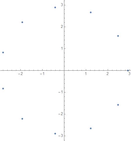
ListPolarPlot[results]