1
$\begingroup$

I am trying to fit data from a simulation to a particular class of polynomials, according to least squares approach.

data = Import["Mathematica file.txt", "Table"]

The polynomials are the shifted Chebyshev polynomials, that is: $${\displaystyle T_{n}^{*}(x)=T_{n}(2x-1)~.}$$ How could one use Mathematica to find the coefficients $a_0$, $a_1$ and so on in: $$\sum_{n=0}^N a_n T_{n}(2x-1)$$ which fits the imported data? Is there a way in Mathematica to find the goodness of fit in Mathematica?

$\endgroup$
1
  • 1
    $\begingroup$ We can use NMinimize to minimize norm of difference between data and approximation with respect to $a_n$. Better you show example of data. $\endgroup$ Commented Apr 6, 2021 at 11:24

2 Answers 2

3
$\begingroup$
Clear["Global`*"]

f[x_] = x*Sin[x];

data = Table[{x, f[x]}, {x, 0, 10, 0.5}];

model[m_, x_] := Sum[a[n] ChebyshevT[n, 2 x - 1], {n, 0, m}];

nlm[m_Integer?Positive, x_] :=
 NonlinearModelFit[data, model[m, x], Array[a, m + 1, 0], x]

Manipulate[
 Module[{model = nlm[m, x]},
  Column[{
    Plot[Evaluate@{f[x], model // Normal}, {x, 0, 10},
     PlotRange -> Full,
     ImageSize -> 300,
     Epilog -> {Red, AbsolutePointSize[4], Point[data]},
     PlotLegends -> Placed[{"f[x]", "approx"}, {.475, .7}]],
    model["ParameterTable"]},
   Alignment -> Center,
   ItemSize -> {35, Automatic}]],
 {{m, 4}, 1, 8, 1, ControlType -> SetterBar}]

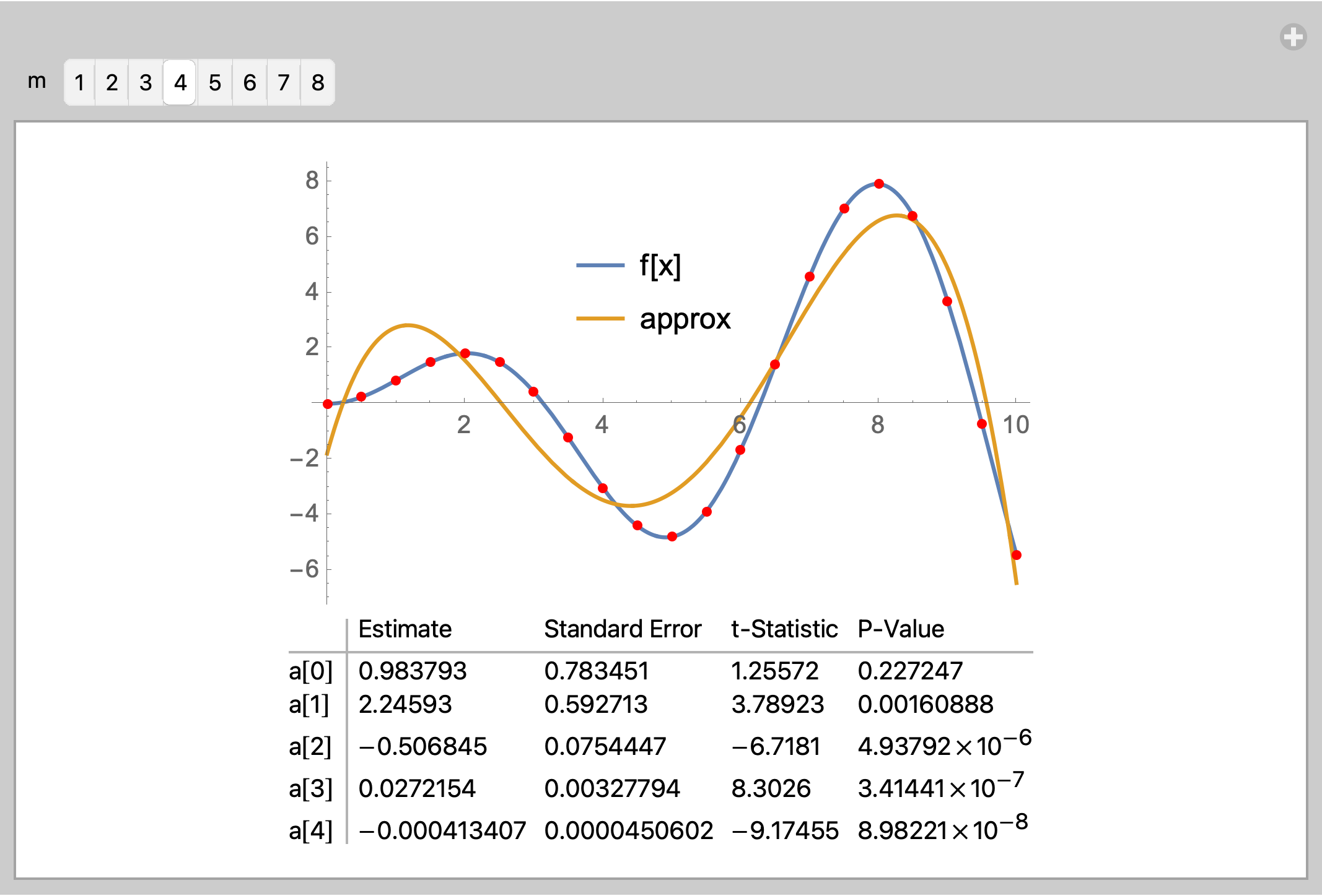
enter image description here

EDIT: The unformatted array of values from the table are

nlm[4, x]["ParameterTableEntries"]

(* {{0.983793, 0.783451, 1.25572, 0.227247}, 
 {2.24593, 0.592713, 3.78923, 0.00160888}, 
 {-0.506845, 0.0754447, -6.7181, 4.93792*10^-6}, 
 {0.0272154, 0.00327794, 8.3026, 3.41441*10^-7}, 
 {-0.000413407, 0.0000450602, -9.17455, 8.98221*10^-8}} *)
$\endgroup$
3
  • $\begingroup$ Thank you! Could you tell me how can I export the parameter table please? $\endgroup$
    – Mark
    Commented Apr 7, 2021 at 10:35
  • $\begingroup$ Use "ParameterTableEntries" (see edit) $\endgroup$
    – Bob Hanlon
    Commented Apr 7, 2021 at 15:16
  • $\begingroup$ @Mark You can use LinearModelFit as well: ts[n_Integer, x_?NumericQ] := ChebyshevT[n, 2 x - 1]; Format[ts[n_, x_]] := Subsuperscript[HoldForm[T], n, "*"][x]; (* Format optional *) model[m_, x_] := Table[ts[n, x], {n, m}]; nlm[m_Integer?Positive, x_] := LinearModelFit[data, model[m, x], x] $\endgroup$
    – Michael E2
    Commented Apr 7, 2021 at 16:26
1
$\begingroup$

Shifted Chebyshev polynomials are orthogonal on {0,1} with the weight function 1/Sqrt[x-x^2].

As the data: dat is not known, but we can create an interpolating function:

fun[x_]=Interpolation[dat]

For an example, we choose funx[x_]=Sin[2Pi x]. We can now expand this function in a series of shifted Chebyshev polynomials. The expansion coefficients are given by:

Clear[sT, fun, c, approx]
sT[n_, x_] := ChebyshevT[n, 2 x - 1]
fun[x_] := Sin[2 Pi x];
c[n_] := NIntegrate[fun[x] sT[n, x]/Sqrt[x - x^2], {x, 0, 1}]/
    NIntegrate[sT[n, x]^2/Sqrt[x - x^2], {x, 0, 1}] // Simplify // Chop

The partial sum tp to n:

approx[n_, x_] := Sum[c[i] sT[i, x], {i, 0, n}] // Quiet

I put a quiet at the end, because this will eventually give some warnings about precision and convergence if, due to symmetry, some coefficients are zero. But these can mostly be ignored. If you want exact results, you may use "Integrate", but this may take a long time.

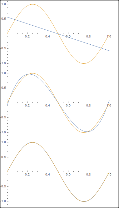
We can now create the first few partial sums and plot them against the original function:

Do[
 f[x_] = approx[i, x];
 Plot[{f[x], fun[x]}, {x, 0, 1}] // Print
 , {i, 1, 5, 2}]

enter image description here

$\endgroup$

Your Answer

By clicking “Post Your Answer”, you agree to our terms of service and acknowledge you have read our privacy policy.

Not the answer you're looking for? Browse other questions tagged or ask your own question.