I have a set of data, where I'd like to find the order of the polynomial that approximates the data, and also know what the Least squares is.
My data:
mydata={{30., 330.579}, {30.1, 326.98}, {30.2, 325.764}, {30.3,
  311.321}, {30.4, 284.364}, {30.5, 316.126}, {30.6, 298.781}, {30.7,
  294.901}, {30.8, 272.735}, {30.9, 268.916}, {31., 289.105}, {31.1,
  269.206}, {31.2, 264.915}, {31.3, 266.102}, {31.4, 247.691}, {31.5,
  269.225}, {31.6, 237.507}, {31.7, 243.386}, {31.8, 244.549}, {31.9,
  227.996}, {32., 219.76}, {32.1, 225.659}, {32.2, 213.498}, {32.3,
  204.988}, {32.4, 209.632}, {32.5, 205.647}, {32.6, 196.185}, {32.7,
  212.885}, {32.8, 190.335}, {32.9, 181.173}, {33., 180.167}, {33.1,
  161.973}, {33.2, 172.964}, {33.3, 166.16}, {33.4, 158.963}, {33.5,
  156.729}, {33.6, 165.902}, {33.7, 149.723}, {33.8, 153.449}, {33.9,
  138.211}, {34., 149.906}, {34.1, 135.848}, {34.2, 121.235}, {34.3,
  128.755}, {34.4, 112.94}, {34.5, 110.743}, {34.6, 126.014}, {34.7,
  108.869}, {34.8, 120.106}, {34.9, 115.747}, {35., 104.896}, {35.1,
  97.7707}, {35.2, 101.916}, {35.3, 106.835}, {35.4, 98.4623}, {35.5,
  91.2834}, {35.6, 79.0194}, {35.7, 84.4551}, {35.8, 80.7674}, {35.9,
  92.3399}, {36., 84.6718}, {36.1, 83.8532}, {36.2, 77.6169}, {36.3,
  73.0614}, {36.4, 76.7545}, {36.5, 77.824}, {36.6, 54.9666}, {36.7,
  72.2144}, {36.8, 61.6352}, {36.9, 58.8691}, {37., 71.0184}, {37.1,
  59.047}, {37.2, 62.543}, {37.3, 50.5073}, {37.4, 50.0954}, {37.5,
  51.4783}, {37.6, 49.1749}, {37.7, 44.4528}, {37.8, 57.2066}, {37.9,
  52.8937}, {38., 51.6243}, {38.1, 50.2519}, {38.2, 42.1921}, {38.3,
  43.7001}, {38.4, 36.1474}, {38.5, 54.591}, {38.6, 59.4826}, {38.7,
  38.8052}, {38.8, 38.2085}, {38.9, 48.2973}, {39., 31.7328}, {39.1,
  34.4054}, {39.2, 58.3053}, {39.3, 51.7763}, {39.4, 51.1076}, {39.5,
  41.9908}, {39.6, 37.1393}, {39.7, 48.3501}, {39.8, 59.6842}, {39.9,
  28.208}, {40., 36.0402}, {40.1, 37.8059}, {40.2, 43.7093}, {40.3,
  59.0266}, {40.4, 41.977}, {40.5, 41.1998}, {40.6, 34.4874}, {40.7,
  36.4598}, {40.8, 45.7132}, {40.9, 42.5813}, {41., 55.5001}, {41.1,
  45.6231}, {41.2, 42.7797}, {41.3, 34.9816}, {41.4, 59.9555}, {41.5,
  59.1558}, {41.6, 58.1503}, {41.7, 50.0516}, {41.8, 58.8706}, {41.9,
  53.63}, {42., 64.3079}, {42.1, 73.0313}, {42.2, 50.954}, {42.3,
  70.9397}, {42.4, 57.6454}, {42.5, 68.1575}, {42.6, 55.2259}, {42.7,
  80.7216}, {42.8, 74.3722}, {42.9, 70.1185}, {43., 85.038}, {43.1,
  69.8574}, {43.2, 98.6267}, {43.3, 72.675}, {43.4, 90.1846}, {43.5,
  85.838}, {43.6, 89.8398}, {43.7, 87.8715}, {43.8, 96.5692}, {43.9,
  94.8867}, {44., 93.2906}, {44.1, 107.817}, {44.2, 110.883}, {44.3,
  113.482}, {44.4, 110.891}, {44.5, 125.85}, {44.6, 117.684}, {44.7,
  120.996}, {44.8, 109.709}, {44.9, 123.845}, {45., 121.603}, {45.1,
  133.1}, {45.2, 124.626}, {45.3, 157.}, {45.4, 128.777}, {45.5,
  152.501}, {45.6, 141.194}, {45.7, 164.115}, {45.8, 158.063}, {45.9,
  162.978}, {46., 167.955}, {46.1, 173.832}, {46.2, 175.932}, {46.3,
  179.225}, {46.4, 194.457}, {46.5, 187.11}, {46.6, 184.621}, {46.7,
  196.59}, {46.8, 193.341}, {46.9, 229.232}, {47., 217.943}, {47.1,
  212.923}, {47.2, 214.198}, {47.3, 213.599}, {47.4, 228.405}, {47.5,
  219.229}, {47.6, 227.861}, {47.7, 236.055}, {47.8, 251.976}, {47.9,
  244.459}, {48., 263.105}, {48.1, 258.907}, {48.2, 276.987}, {48.3,
  260.376}, {48.4, 273.986}, {48.5, 285.245}, {48.6, 282.607}, {48.7,
  280.599}, {48.8, 299.848}, {48.9, 312.727}, {49., 309.721}, {49.1,
  302.612}, {49.2, 325.601}, {49.3, 318.055}, {49.4, 330.583}, {49.5,
  336.413}, {49.6, 332.563}, {49.7, 357.118}, {49.8, 356.767}, {49.9,
  351.579}, {50., 378.437}}
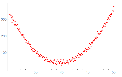
I started with plotting:
My idea was then to create a Table containing exponentials (1, x, x^2, x^3...), and fit a function using the Fit method.
expo[n_] := Table[x^k, {k, 0, n}]
approx = Fit[mydata, expo[5], x] #example using order 5
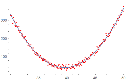
Visualizing my result (here with order=5):
Show[dataplott, Plot[approx, {x, 30, 50}]]
If my approach is correct, I don't know how to incorporate a range of evaluation numbers and see which is the best.
I also have been looking a bit at the Interpolation method:
interapprox = Interpolation[mydata]
interplot = Plot[interapprox[\[FormalX]], {\[FormalX], 30., 50.},
  PlotStyle -> Gray]
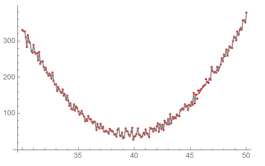
Show[dataplott, interplot]
This gives me an approximation output that looks pretty nice, but the InterpolationOrder seems to be default=3, so I'm not sure if this actually works (or perhaps how it works).
Output:
Preferably I'm seeking a solution that also lets me get the Least Squares.
I might add that I'm rather new to linear algebra & mathematica, so apologies for any blunders. Ciao.

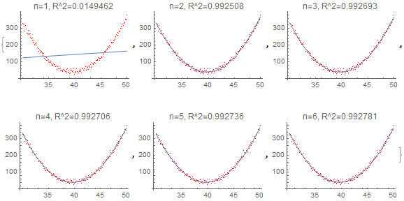
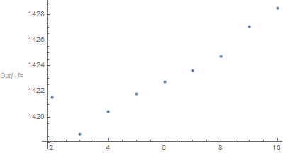
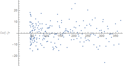
LinearModelFitis what you want. And @DanielHuber 's comment is also critical as a "good" fit depends on the subject matter and your objectives. You might consider asking this on stats.stackexchange.com because having a justifiable decision process is more of a statistical question rather than a Mathematica question. $\endgroup$