8
$\begingroup$

Is it possible to find or construct a RegionPlot out of KnotData? My motivation is to Texture the knots as per here.

After much searching and playing around, I found this, which frustratingly doesn't give the equations for the inTinftube and onTinftube functions.

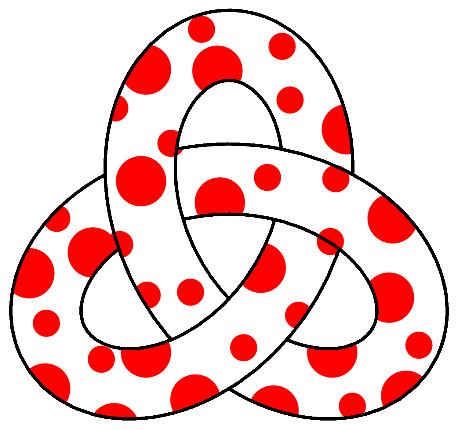
Desired output is something like this (but in 3D):

$\endgroup$

4 Answers 4

9
$\begingroup$

Edit

n = 15;
vor = VoronoiMesh[
   RandomPoint[Rectangle[{0, 0}, {2 π, 2 π}], 
    n], {{0, 2 π}, {0, 2 π}}];
polys = MeshPrimitives[vor, 2];
g = Show[Table[{Red, 
      Disk[x /. Last[#], Abs@First[#]] &@
       NMinimize[SignedRegionDistance[poly][x], 
        x ∈ poly]}, {poly, polys}] // Graphics];
curve3 = KnotData["Trefoil", "SpaceCurve"];
basis = Last[FrenetSerretSystem[curve3[t], t]];
{tangent, normal, binormal} = basis;
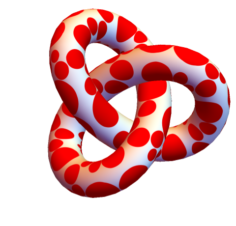
ParametricPlot3D[
 curve3[t] + .6 (Cos[u]*normal + Sin[u]*binormal), {u, 0, 
  2 π}, {t, 0, 2 π}, PlotPoints -> 80, Mesh -> None, 
 Boxed -> False, Axes -> False, PlotStyle -> Texture[g], 
 TextureCoordinateScaling -> True, 
 TextureCoordinateFunction -> Function[{x, y, z, u, t}, {u, 9 t}], 
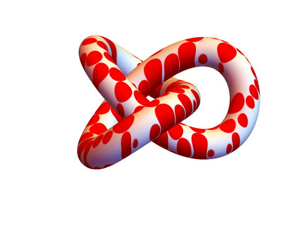
 ViewPoint -> {0.2, -0.3, 3.3}]

enter image description here

Original

A starting point.

curve3 = KnotData["Trefoil", "SpaceCurve"];
basis = Last[FrenetSerretSystem[curve3[t], t]];
{tangent, normal, binormal} = basis;
g = Graphics[{Red, Disk[{0, 0}, .5]}, PlotRangePadding -> .5];
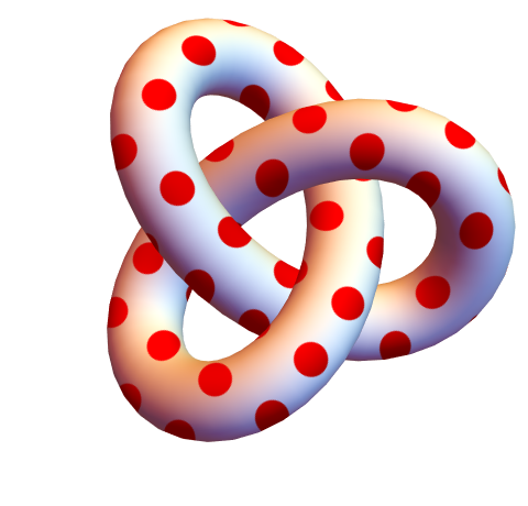
ParametricPlot3D[
 curve3[t] + .6 (Cos[u]*normal + Sin[u]*binormal), {u, 0, 
  2 π}, {t, 0, 2 π}, PlotPoints -> 80, Mesh -> None, 
 Boxed -> False, Axes -> False, PlotStyle -> Texture[g], 
 TextureCoordinateScaling -> False, 
 TextureCoordinateFunction -> Function[{x, y, z, t, u}, {x, y}], 
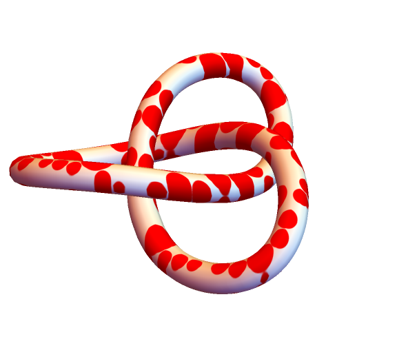
 ViewPoint -> {0.2, -0.3, 3.3}]

enter image description here

$\endgroup$
1
  • $\begingroup$ fantastic - thanks! $\endgroup$
    – martin
    Commented Feb 26, 2021 at 15:49
8
$\begingroup$

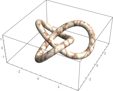
You can feed the BoundaryMeshRegion[] you can obtain from KnotData[] into RegionPlot3D[]. For example:

trefBMR = KnotData["Trefoil", "BoundaryMeshRegion"];
RegionPlot3D[RegionMember[trefBMR, {x, y, z}],
             {x, -7/2, 7/2}, {y, -7/2, 7/2}, {z, -3/2, 3/2},
             BoxRatios -> Automatic, Lighting -> "Neutral",
             Mesh -> None, PlotPoints -> 35, 
             PlotStyle -> Directive[Texture[ExampleData[{"ColorTexture",
                                                         "WhiteMarble"}]]]]

marbled knot

$\endgroup$
2
  • $\begingroup$ Thank you, this is great. Is it possible to vary the thickness of the knot? $\endgroup$
    – martin
    Commented Feb 26, 2021 at 15:24
  • 1
    $\begingroup$ It's a little harder to do, but certainly doable. (You'll have to wait a bit for it, as I am currently evaluating something else.) $\endgroup$ Commented Feb 26, 2021 at 16:43
7
$\begingroup$

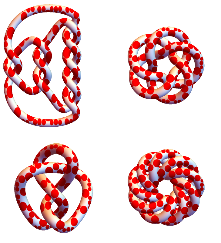
enter image description here

Multicolumn[Graphics3D[{SurfaceAppearance["TextureShading", Texture[disks]], 
     Tube[BSplineCurve[KnotData[#, "SpaceCurve"] /@ Subdivide[0, 2 Pi, 100], 
       SplineClosed -> True], .4]}, 
    Boxed -> False, ImageSize -> Medium, ViewPoint -> {0, 0, 5}] & /@ 
 {{"PretzelKnot", {5, 3, 2}}, "FigureEight",
  {"TorusKnot", {3, 5}}, {"TorusKnot", {4, 9}}}, 2] 

Update: In versions 12.1+, we can use the directive SurfaceAppearance["TextureShading", Texture[img]] to texturize any surface with img:

reg = TriangulateMesh[BoundaryDiscretizeRegion[Rectangle[]], MaxCellMeasure -> .02];

disks = Graphics[{Red, MeshPrimitives[reg, 2] /. Polygon -> (Apply[Disk] @* Insphere)}];

 Graphics3D[{SurfaceAppearance["TextureShading", Texture[disks]], 
   KnotData["Trefoil", "ImageData"]}, 
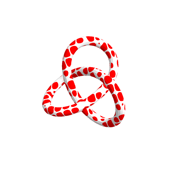
  Boxed -> False, ImageSize -> Large] 
enter image description here

We can construct a Tube with the desired radius using KnotData["Trefoil", "SpaceCurve"]:

Graphics3D[{SurfaceAppearance["TextureShading", Texture[disks]], 
  Tube[BSplineCurve[KnotData["Trefoil", "SpaceCurve"] /@ Subdivide[0, 2 Pi, 100], 
    SplineClosed -> True], .5]}, 
 Boxed -> False, ImageSize -> Large] 
enter image description here

Alternatively, we can use SurfaceAppearance["TextureShading", Texture[disks]] as the setting for PlotStyle in ParametricPlot3D in cvgmt's answer:

ParametricPlot3D[curve3[t] + .6 (Cos[u] normal + Sin[u] binormal), 
 {u, 0, 2 π}, {t, 0, 2 π}, PlotPoints -> 80, Mesh -> None, 
 Boxed -> False, Axes -> False, 
 PlotStyle -> SurfaceAppearance["TextureShading", Texture[disks]], 
 ViewPoint -> {0.2, -0.3, 3.3}, Lighting->"Neutral"]
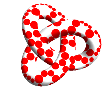
enter image description here

Original answer:

We can use the new-in-12.1 directive HalfToneShading:

Graphics3D[{HalftoneShading[#, Red], KnotData["Trefoil", "ImageData"]}, 
 Lighting -> "Neutral", ImageSize -> 250, Boxed -> False, 
    ViewPoint -> {1.5, -1.5, 4.}] & /@ {.3, .5, .7} // Row 
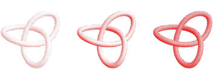
enter image description here

Needless to say, this approach is not match for cvgmt's approach in terms of flexibility and beauty of the pictures produced.

To get some flexibility in controlling the density of shapes, we can use the options of SurfaceAppearance to define a directive with options:

Options[surfaceAppearance] = {"StepCount" -> 1, "Tiling" -> {5, 5}, 
   "FeatureColor" -> Red, "UseScreenSpace" -> 0, "IsTwoTone" -> 1, 
   "LuminanceModifier" -> 0.0, "Shape" -> "Disk"};

surfaceAppearance[opts : OptionsPattern[surfaceAppearance]] := 
 SurfaceAppearance["RampShading", 
  Sequence @@ FilterRules[{opts, Options[surfaceAppearance]}, Except["Shape"]], 
  "Arguments" -> {"HalftoneShading", 0.5, Red, OptionValue["Shape"]}, 
  EdgeForm[], Texture["HalftoneShading" <> OptionValue["Shape"]]]

Examples:

Graphics3D[{surfaceAppearance[], KnotData["Trefoil", "ImageData"]},
  Lighting -> "Accent", Boxed -> False, ViewPoint -> {1.5, -1.5, 4.}]
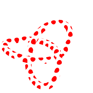
enter image description here

Use surfaceAppearance["Tiling" -> {15, 15}] to get:
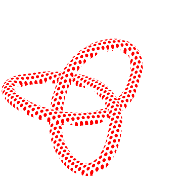
enter image description here

Use surfaceAppearance["UseScreenSpace" -> 1, "StepCount" -> 2, "Tiling" -> {7, 7}] to get:
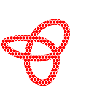
enter image description here

Use surfaceAppearance["Tiling" -> {15, 15}, "Shape"->"Triangle"] to get:
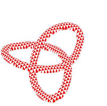
enter image description here

Use surfaceAppearance["StepCount" -> 3,"Tiling" -> {10,10},"Shape" -> "Hexagon"] to get:

enter image description here

$\endgroup$
1
  • $\begingroup$ brilliant - thankyou! had no idea this existed :) $\endgroup$
    – martin
    Commented Mar 1, 2021 at 11:58
5
$\begingroup$
SliceContourPlot3D[Sin[5 x] Sin[6 y] Sin[4 z], 
 KnotData["Trefoil", "Region"],
 {x, -Pi, Pi}, {y, -Pi, Pi}, {z, -Pi, Pi}, 
 Contours -> {-1/6, 1/6}, ContourStyle -> None, 
 ContourShading -> {White, Red}, 
 Boxed -> False, ImageSize -> Large, Axes -> False, PlotPoints -> 90]

enter image description here

$\endgroup$

Your Answer

By clicking “Post Your Answer”, you agree to our terms of service and acknowledge you have read our privacy policy.

Not the answer you're looking for? Browse other questions tagged or ask your own question.