7
$\begingroup$

Context to understand the question

Suppose that I have the next equation

sol = ParametricNDSolve[{y'[t] == a y[t], y[0] == 1}, y, {t, 0, 10}, {a}]

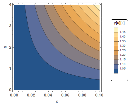
And I make a Contour Plot of this equation

 ContourPlot[y[a][x] /. sol, {x, 0, 0.1}, {a, 0, 4},PlotLegends -> BarLegend[Automatic,LegendMarkerSize -> 180,   LegendFunction -> "Frame", LegendMargins -> 5, LegendLabel -> "y[a][x]"], Frame -> True,  FrameLabel -> {{"a", ""}, {"x", ""}}, BaseStyle -> {FontWeight -> "Bold", FontSize -> 14}]

enter image description here

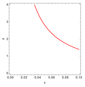
Next I obtain a specific line of this ContourPlot

ContourPlot[y[a][x] /. sol, {x, 0, 0.1}, {a, 0, 4}, Frame -> True, FrameLabel -> {{"a", ""}, {"x", ""}},  BaseStyle -> {FontWeight -> "Bold", FontSize -> 14}, 
Contours -> {1.15}, ContourStyle -> Directive[Thick, Red], 
ContourShading -> None]

enter image description here

Quesiton

Is there an "easy" way to obtain an equation for the red line, I mean the function $a(x)$?

I need the function, to make calculations, for example $(a(x))^{1/2}$.

"Long" way to obtain the equation for the red line

I usually take a image of the the graph and use webplotdigitizer to extrac the points of the graph and after I aproximate the extracted points with a polinominal function, however this prodedure can be slow.

$\endgroup$
1
  • $\begingroup$ A contour is just a level set, also known as an isoline - a curve where $f(x) = c$ for some value $c$. If you can solve that equation you can parametrize the curve. $\endgroup$
    – flinty
    Commented Jun 6, 2020 at 22:56

3 Answers 3

8
$\begingroup$

What you may not know is that the notebook interface is a bit like a web browser. Whatever complicated interface the web browser is showing, you can always just right-click and show the HTML source code for it. It's not delivered as a bunch of pixels, and similarly, graphics (to be distinguished from actual images, including rasterized graphics) are just expressions. Consequently, you don't need to use a third-part tool to get the coordinates of the line. Just do it like this:

sol = ParametricNDSolve[{y'[t] == a y[t], y[0] == 1}, y, {t, 0, 10}, {a}];
cp = ContourPlot[y[a][x] /. sol, {x, 0, 0.1}, {a, 0, 4}, Contours -> {1.15}];
line = First@Cases[Normal[cp], _Line, Infinity];

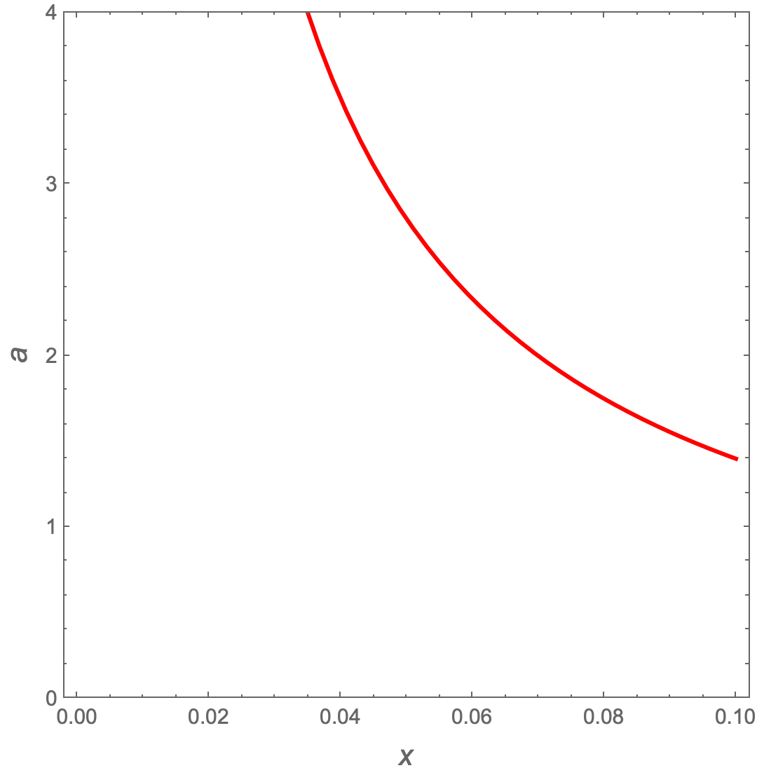
Visualizing it to make sure it's working:

Graphics[{line}, PlotRange -> {{0, 0.1}, {0, 4}}, AspectRatio -> 1]

Output

It seems like you already have a way forward from this point with polynomial fitting that you have done previously.

Normal is needed because in the expression generated by ContourPlot, the line coordinates are encoded with GraphicsComplex. I use Normal to replace the coordinate indices with the actual coordinates.

I might also add that the functionality offered by the third-party tool you mention seems to be similar to a function already built into Mathematica. You can right-click the graphics in Mathematica and click "get coordinates". You can then left-click on a couple of points along the line and press ctrl+c to copy the points to clipboard. Now you can paste that data into another cell.

$\endgroup$
5
  • $\begingroup$ Really impresive solution. However there is something that I don't understand, how I can I get "line" as a function of "x"? In the past when I need to make manipulations I just use the function $a[x]$, for example if I do $2*a[0.1]$ I get a number, I tried with $2*line[0.1]$, but doesn't work. $\endgroup$
    – No name
    Commented Jun 7, 2020 at 0:17
  • 1
    $\begingroup$ @Cruz I’m not showing that part. Line is a graphics primitive. You can turn it into a list using List @@. You can use Interpolation or whatever to get a function, or as I said in my answer, the polynomial fitting approach that you’ve used so far should also be possible to use with these coordinates. I focused on getting the coordinates, since that seemed to be the main problem. $\endgroup$
    – C. E.
    Commented Jun 7, 2020 at 0:29
  • $\begingroup$ Thank you, is one of the problems. But I was looking for the function. $\endgroup$
    – No name
    Commented Jun 7, 2020 at 0:30
  • 1
    $\begingroup$ @Cruz ok, then I recommend Interpolation. $\endgroup$
    – C. E.
    Commented Jun 7, 2020 at 0:32
  • $\begingroup$ {minx, maxx} = MinMax[line[[1]][[All, 1]]]; func = Interpolation[Midpoint /@ Partition[line[[1]], 2, 1]]; Plot[func[x], {x, minx, maxx}] - it's up to you if you want to use the Midpoints of the lines that make up the curve - you could also choose points on the end of the line. Or you could even get points randomly like RandomPoint[line,1000] and then fit a curve. $\endgroup$
    – flinty
    Commented Jun 7, 2020 at 12:22
6
$\begingroup$

For this specific case the exact solution can be found.

Clear["Global`*"]

eqns = {y'[t] == a y[t], y[0] == 1};

sol = DSolve[eqns, y, t][[1]]

(* {y -> Function[{t}, E^(a t)]} *)

Verifying the solution,

eqns /. sol

(* {True, True} *)

a[x_, const_] = a /. Solve[(y[x] /. sol) == const, a][[1]] /. C[1] -> 0

(* Log[const]/x *)

With[{const = 1.15},
 Plot[a[x, const], {x, 0, 0.1},
  PlotRange -> {0, 4},
  AspectRatio -> 1,
  PlotStyle -> Directive[Thick, Red],
  Frame -> True,
  FrameLabel -> (Style[#, 14] & /@ {x, a})]]

enter image description here

$\endgroup$
3
$\begingroup$

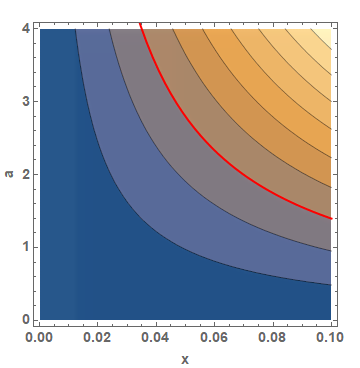
My method is uglier than just extracting a spline like with C. E's answer. It's possible find points on this contour with an NMinimize and use an Interpolation to get the curve as a function of $x$ (see func below):

sol = ParametricNDSolve[{y'[t] == a y[t], y[0] == 1}, 
   y, {t, 0, 10}, {a}];
fn = y /. sol;

(* Set the target contour *)
target = 1.15;

(* For each value of 'a' find 'x' that minimizes square error of fn[a][x] to target *)
minpoints = Table[
  {x /. Last[NMinimize[{(fn[a][x] - target)^2, 0 < x < 0.1}, x]], a}, {a, 0, 4, .1}
];

(* Choose the best {x,a} solution points closest (within 10^-6) to the target value *)
filteredMinpoints = Select[minpoints, Abs[fn[#[[2]]][#[[1]]] - target] < 10^-6 &];

(* Interpolate this curve - this is now a function of 'x' we can use later *)
func = Interpolation[filteredMinpoints];
Show[
 ContourPlot[y[a][x] /. sol, {x, 0, 0.1}, {a, 0, 4}, 
  PlotLegends -> 
   BarLegend[Automatic, LegendMarkerSize -> 180, 
    LegendFunction -> "Frame", LegendMargins -> 5, 
    LegendLabel -> "y[a][x]"], Frame -> True, 
  FrameLabel -> {{"a", ""}, {"x", ""}}, 
  BaseStyle -> {FontWeight -> "Bold", FontSize -> 14}],

 (* Show a plot of the curve we interpolated *)
 Plot[Quiet@func[x], {x, 0, .1}, PlotStyle -> {Red, Thick}]
]

contour curve

$\endgroup$
3
  • $\begingroup$ I have two questions. First, why this solution is computaninaly "slow"? And second, when you compile your code it says "InterpolatingFunction::dmval: Input value {2.04286*10^-6} lies outside the range of data in the interpolating function. Extrapolation will be used." what is the meaning of this? $\endgroup$
    – No name
    Commented Jun 7, 2020 at 0:26
  • $\begingroup$ Oh sorry, I don't know if is too much. But I really want to understand why you use "fn = y /. sol", is incorrect if I do "fn[x_]:=y[x] /. sol"? $\endgroup$
    – No name
    Commented Jun 7, 2020 at 0:29
  • 1
    $\begingroup$ 1) It's slow because it's doing a minimization for every point. If you want a fast method use the analytic solution with DSolve or extract the spline from the plot. I'm leaving this method here because it's an alternative when DSolve isn't feasible. 2) At the edges it's plotting an interpolation beyond the points I gave it, so it needs to extrapolate. 3) I use fn = y /. sol because your original ParametricNDSolve returns a rule y -> .... $\endgroup$
    – flinty
    Commented Jun 7, 2020 at 1:27

Your Answer

By clicking “Post Your Answer”, you agree to our terms of service and acknowledge you have read our privacy policy.

Not the answer you're looking for? Browse other questions tagged or ask your own question.