6
$\begingroup$

What's the fastest way to find the local maxima of a 2D list? E.g.

nx = ny = 100;
dat = Table[Sin[2. \[Pi] x/nx] (0.1 + Cos[2. \[Pi] y/ny]), {y, 0, ny}, {x, 0, nx}];

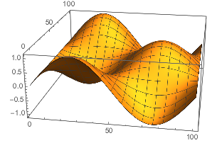
ListPlot3D[dat]
Mathematica graphics

This (updated) function has three local maxima of different heights:

Position[MaxDetect[dat], 1]
(* {{1, 26}, {51, 76}, {101, 26}} *)

dat[[1, 26]]
dat[[51, 76]]
dat[[101, 26]]
(* 1.1, 0.9, 1.1 *)

My original attempt was super-slow:

RepeatedTiming[MaxDetect[Chop@dat];][[1]]
(* 1.55 *)

Turns out using Chop is a very bad idea. Without it is 100X faster:

RepeatedTiming[MaxDetect[dat];][[1]]
(* 0.016 *)

Along the way I discovered another version that is 2X faster yet:

RepeatedTiming[MaxDetect[Image[dat]];][[1]]
(* 0.0067 *)

Questions

  1. Why is MaxDetect so much slower when Chop is applied? (I should add that my actual non-example problem has lots of small values that needed to Chop-ping)
  2. Why does converting to an Image speed it up further?
  3. Is there any faster way available?
$\endgroup$
3
  • 4
    $\begingroup$ how about UnitStep[dat - Max[dat]]? $\endgroup$
    – kglr
    Commented Sep 22, 2019 at 9:29
  • 1
    $\begingroup$ also Chop[dat, Max@dat] $\endgroup$
    – kglr
    Commented Sep 22, 2019 at 9:46
  • 2
    $\begingroup$ I see now that my toy example was too simplistic. In my real problem, not all local maxima are equal, so this approach doesn't work. Let me adjust the question. Sorry! $\endgroup$
    – Chris K
    Commented Sep 22, 2019 at 9:51

4 Answers 4

9
$\begingroup$

Why is MaxDetect so much slower when Chop is applied?

Because Chop returns exact zeros what prevents packing of the matrix attempted by MaxDetect. You can detect an attempt to pack the array with Trace:

Trace[MaxDetect[{{1.}}], Developer`ToPackedArray] // Flatten

screenshot

Applying N after Chop gives almost the same speed as without Chop because now the matrix can be packed again:

RepeatedTiming[MaxDetect[dat];][[1]]
RepeatedTiming[MaxDetect[N@Chop@dat];][[1]]
0.06
0.07

Why does converting to an Image speed it up further?

It seems that MaxDetect is simply not so well-optimized for an array input as compared to an Image input. A superficial analysis follows.

  1. Compare the complexity of Trace outputs in the both cases:

    Trace[MaxDetect[dat]] // LeafCount
    Trace[MaxDetect[Image@dat]] // LeafCount
    
    79670996
    260610
    

    It indicates that in the case of array input it is evaluated many times as an (unpacked?) array, while in the case of Image input it is evaluated as an atomic Image object what may be faster.

  2. Additional evidences in support of the previous guess:

    Count[Trace[MaxDetect[dat]], _Image, Infinity]
    Count[Trace[MaxDetect[Image@dat]], _Image, Infinity]
    
    8
    1913
    
    Count[Trace[MaxDetect[dat]], _List?MatrixQ, Infinity]
    Count[Trace[MaxDetect[Image@dat]], _List?MatrixQ, Infinity] // Quiet
    
    7432
    367
    
  3. And finally let us compare how many packed and non-packed array evaluations appear in the both cases:

    Count[Trace[MaxDetect[dat]], a_List /; Developer`PackedArrayQ[a], Infinity]
    Count[Trace[MaxDetect[Image@dat]], a_List /; Developer`PackedArrayQ[a], Infinity] // Quiet
    
    102
    204
    
    Count[Trace[MaxDetect[dat]], a_List /; ! Developer`PackedArrayQ[a], Infinity]
    Count[Trace[MaxDetect[Image@dat]], a_List /; ! Developer`PackedArrayQ[a], Infinity] // Quiet
    
    748562
    8706
    

    From the last output we see that there seems to be about 100 times more evaluations of non-packed arrays in the case of array input as compared to Image input. I think that now the situation is clear enough.

$\endgroup$
1
  • $\begingroup$ A better alternative to N+Chop would be Threshold. That keeps the arrays packed all the time. $\endgroup$ Commented Sep 22, 2019 at 20:43
10
$\begingroup$

Is there any faster way available?

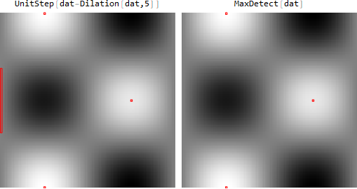
There is, if you're willing to to use a different definition of "local maximum". If a local maximum is any value at least as high as any value in a 11x11 neighborhood, then you can use UnitStep[dat - Dilation[dat, 5]], which is about 16 times faster for your data:

RepeatedTiming[MaxDetect[dat];][[1]]

0.016

RepeatedTiming[UnitStep[dat - Dilation[dat, 5]];][[1]]

0.00101

But the result is slightly different:

enter image description here

Note the marked pixels on the left border in the dat-Dilation version. By the definition above, these pixels mark one extended local maximum.

$\endgroup$
1
  • $\begingroup$ Conversion to 64-bit floating point numbers doesn't increase the speed significantly: try RepeatedTiming[MaxDetect[Image[dat, "Real64"]];][[1]]. $\endgroup$ Commented Sep 22, 2019 at 16:12
8
$\begingroup$

A severe problem is that Table generates an unpacked array, a thing that is often very annoying. When converting to an image, it is packed automatically (one can check that, e.g., with Developer`PackedArrayQ[ImageData[Image[dat]]]). And because many functions work faster on packed arrays than on unpacked ones, this increases the performance.

A vectorized implementation that exploits the very nature of the function (and is thus not very generalizable) is the following:

nx = ny = 1000;
dat = KroneckerProduct[
     (0.1 + Cos[Subdivide[0., 2. Pi, ny]]),
     Sin[Subdivide[0., 2. Pi, nx]]
     ];

0.003691

The maxima can be found by comparing each value to the maximum of its neighbors. The latter can be done efficiently with MaxFilter:

getindex = {Quotient[#, Dimensions[dat][[1]]] + 1, Mod[#, Dimensions[dat][[2]], 1]} &;
idx = getindex /@ 
     Random`Private`PositionsOf[
      Flatten@UnitStep[dat - MaxFilter[dat, {1, 1}]], 
      1
      ]; // AbsoluteTiming // First
idx
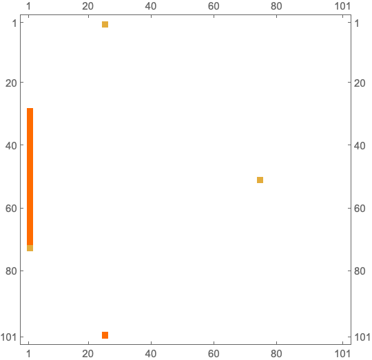
MatrixPlot@SparseArray[idx -> 1, Dimensions[dat]]

0.00108

{{1, 26}, {29, 1}, {30, 1}, {31, 1}, {32, 1}, {33, 1}, {34, 1}, {35, 1}, {36, 1}, {37, 1}, {38, 1}, {39, 1}, {40, 1}, {41, 1}, {42, 1}, {43, 1}, {44, 1}, {45, 1}, {46, 1}, {47, 1}, {48, 1}, {49, 1}, {50, 1}, {51, 1}, {51, 76}, {52, 1}, {53, 1}, {54, 1}, {55, 1}, {56, 1}, {57, 1}, {58, 1}, {59, 1}, {60, 1}, {61, 1}, {62, 1}, {63, 1}, {64, 1}, {65, 1}, {66, 1}, {67, 1}, {68, 1}, {69, 1}, {70, 1}, {71, 1}, {72, 1}, {73, 1}, {101, 26}}

enter image description here

This is about 10 times faster than MaxDetect. But it does not distinguish between local maxima and strict local maxima. However, a second sweep over the local maxima (which is much less expensive) could filter out the strict local maxima.

$\endgroup$
2
  • 1
    $\begingroup$ The OP has changed the problem in a breaking way in his last edit, so the solutions by kglr and Ulrich are no more acceptable: he states that the function may have several local maxima with different heights. I do not know how best to behave in this situation: such a change is against the rules of the site (as I understand). $\endgroup$ Commented Sep 22, 2019 at 16:56
  • 1
    $\begingroup$ @AlexeyPopkov Oh my, you are right. Well, I changed my answer towards the new question. $\endgroup$ Commented Sep 22, 2019 at 17:16
6
$\begingroup$

A little bit faster than @kglr 's tricky answer is

Position[dat, Max[dat]]
$\endgroup$

Your Answer

By clicking “Post Your Answer”, you agree to our terms of service and acknowledge you have read our privacy policy.

Not the answer you're looking for? Browse other questions tagged or ask your own question.