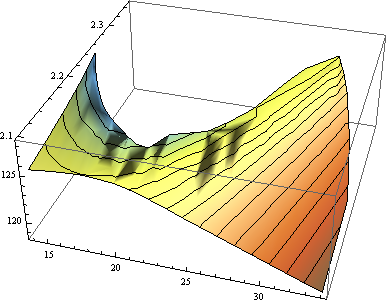
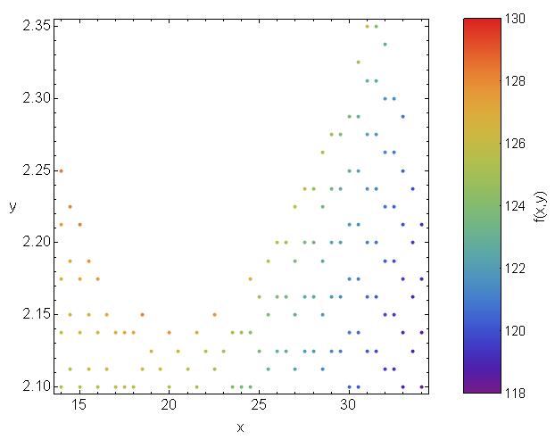
I want to create ListContourPlots for sets of Data (from a physics simulation) given as Triplets {x, y, f(x, y)}. Certain parameter regions in the x-y-plane are excluded by experiments. The list of triplets simply does not contain any Triplets with excluded x-y-parameters. ListPointPlot3D shows that this is not the problem.
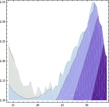
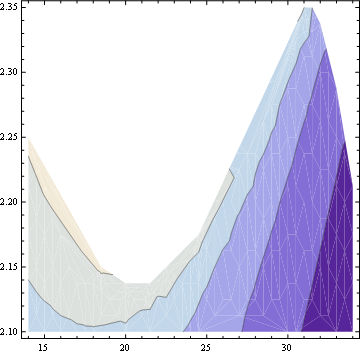
The problem is that ListContourPlot (which I prefer to use, since I have to correlate exclusions from different quantities) interpolates values into regions where no data points are given, as soon as the shape of the data-filled region becomes concave.
I already tried creating a list that is only defined in the excluded regions and painting it over the original plot, however, my dataset is not entirely concave, so that overpainting will cut off some of the interesting parts of the plot...
I figure it has something to do with the "Method" option of ListContourPlot, but those things are really badly documented.
Here is a list of 140 data triplets that show the problem.
l= {{14., 2.1, 125.433}, {14., 2.1375, 125.957}, {14., 2.175,
  126.58}, {14., 2.2125, 127.354}, {14., 2.25, 128.415}, {14.5,
  2.1125, 125.698}, {14.5, 2.15, 126.315}, {14.5, 2.1875,
  127.087}, {14.5, 2.225, 128.152}, {15., 2.1, 125.593}, {15., 2.1375,
   126.238}, {15., 2.175, 127.061}, {15., 2.2125, 128.256}, {15.5,
  2.1125, 125.886}, {15.5, 2.15, 126.669}, {15.5, 2.1875,
  127.783}, {16., 2.1, 125.73}, {16., 2.1375, 126.534}, {16., 2.175,
  127.708}, {16.5, 2.1125, 126.054}, {16.5, 2.15, 127.082}, {17., 2.1,
   125.829}, {17., 2.1375, 126.85}, {17.5, 2.1, 125.858}, {17.5,
  2.1375, 127.016}, {18., 2.1, 125.868}, {18., 2.1375,
  127.185}, {18.5, 2.1125, 126.243}, {18.5, 2.15, 128.277}, {19.,
  2.125, 126.76}, {19.5, 2.1125, 126.183}, {20., 2.1, 125.633}, {20.,
  2.1375, 127.686}, {20.5, 2.125, 126.573}, {21., 2.1125,
  125.763}, {21.5, 2.1, 125.093}, {21.5, 2.1375, 127.062}, {22.,
  2.125, 125.806}, {22.5, 2.1125, 124.979}, {22.5, 2.15,
  127.707}, {23., 2.125, 125.111}, {23.5, 2.1, 124.03}, {23.5, 2.1375,
   125.248}, {24., 2.1, 123.738}, {24., 2.1375, 124.82}, {24.5, 2.1,
  123.445}, {24.5, 2.1375, 124.411}, {24.5, 2.175, 126.896}, {25.,
  2.125, 123.689}, {25., 2.1625, 124.924}, {25.5, 2.1125,
  123.092}, {25.5, 2.15, 123.987}, {25.5, 2.1875, 125.801}, {26.,
  2.125, 123.022}, {26., 2.1625, 123.937}, {26., 2.2, 125.892}, {26.5,
   2.125, 122.703}, {26.5, 2.1625, 123.512}, {26.5, 2.2,
  124.901}, {27., 2.1125, 122.198}, {27., 2.15, 122.848}, {27.,
  2.1875, 123.782}, {27., 2.225, 125.874}, {27.5, 2.125,
  122.095}, {27.5, 2.1625, 122.745}, {27.5, 2.2, 123.676}, {27.5,
  2.2375, 125.734}, {28., 2.125, 121.808}, {28., 2.1625,
  122.394}, {28., 2.2, 123.198}, {28., 2.2375, 124.563}, {28.5,
  2.1125, 121.39}, {28.5, 2.15, 121.87}, {28.5, 2.1875,
  122.506}, {28.5, 2.225, 123.412}, {28.5, 2.2625, 125.253}, {29.,
  2.125, 121.29}, {29., 2.1625, 121.747}, {29., 2.2, 122.372}, {29.,
  2.2375, 123.256}, {29., 2.275, 124.961}, {29.5, 2.125,
  121.036}, {29.5, 2.1625, 121.454}, {29.5, 2.2, 122.006}, {29.5,
  2.2375, 122.762}, {29.5, 2.275, 123.966}, {30., 2.1, 120.465}, {30.,
   2.1375, 120.896}, {30., 2.175, 121.334}, {30., 2.2125,
  121.862}, {30., 2.25, 122.595}, {30., 2.2875, 123.735}, {30.5, 2.1,
  120.187}, {30.5, 2.1375, 120.599}, {30.5, 2.175, 121.065}, {30.5,
  2.2125, 121.525}, {30.5, 2.25, 122.157}, {30.5, 2.2875,
  123.07}, {30.5, 2.325, 124.9}, {31., 2.125, 120.167}, {31., 2.1625,
  120.593}, {31., 2.2, 121.078}, {31., 2.2375, 121.561}, {31., 2.275,
  122.237}, {31., 2.3125, 123.247}, {31., 2.35, 126.014}, {31.5,
  2.125, 119.881}, {31.5, 2.1625, 120.285}, {31.5, 2.2,
  120.747}, {31.5, 2.2375, 121.268}, {31.5, 2.275, 121.808}, {31.5,
  2.3125, 122.628}, {31.5, 2.35, 124.034}, {32., 2.1125,
  119.484}, {32., 2.15, 119.849}, {32., 2.1875, 120.264}, {32., 2.225,
   120.742}, {32., 2.2625, 121.268}, {32., 2.3, 121.85}, {32., 2.3375,
   122.72}, {32.5, 2.1125, 119.213}, {32.5, 2.15, 119.558}, {32.5,
  2.1875, 119.949}, {32.5, 2.225, 120.396}, {32.5, 2.2625,
  120.911}, {32.5, 2.3, 121.431}, {33., 2.1, 118.846}, {33., 2.1375,
  119.16}, {33., 2.175, 119.512}, {33., 2.2125, 119.91}, {33., 2.25,
  120.365}, {33., 2.2875, 120.871}, {33.5, 2.125, 118.783}, {33.5,
  2.1625, 119.101}, {33.5, 2.2, 119.458}, {33.5, 2.2375,
  119.856}, {34., 2.1, 118.333}, {34., 2.1375, 118.614}, {34., 2.175,
  118.923}, {34., 2.2125, 119.261}};

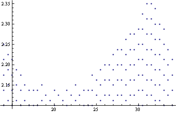
ListPlot@l[[All, 1 ;; 2]]

InterpolationOrder->0is the way to go. @Neuneck If you provide some code for the plot and an image ilustrating the problem (instead of a "spoiler"), you are bound to get better answers. $\endgroup$