I have a set of data
table = Reverse[{
   {0, -947}, {-212, -947}, {-424, -950}, {-635, -963}, {-845, -995}, {-1051, -1044},
   {-1248, -1119}, {-1432, -1224}, {-1591,-1365}, {-1715, -1537}, {-1796, -1732},
   {-1828, -1942}, {-1810,-2153}, {-1755, -2357}, {-1668, -2551}, {-1556, -2730},
   {-1423,-2895}, {-1278, -3050}, {-1126, -3197}, {-973, -3343}, {-803,-3506}
}];
which I need to interpolate with a parametric curve. Endpoints and tangent vectors at them are critical. Trying independent polynomial fits for X and Y leads to a wavy curve which is unacceptable. BSplineFunction of degree around 3 leads to a very good-looking curve:
interp = BSplineFunction[table, SplineDegree -> 3];
Show[ListPlot[table], ParametricPlot[interp[t], {t, 0, 1}], AspectRatio -> 1]
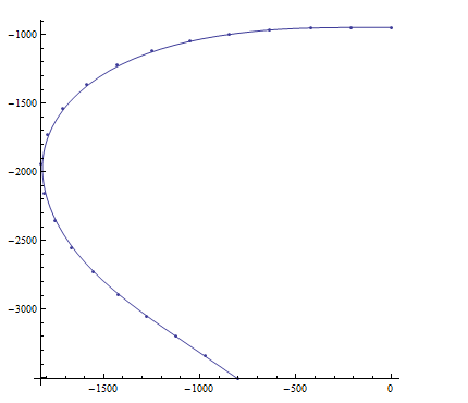
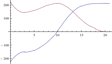
but has a discontinuous derivative (btw: why? help promises that it should be a BSplineFunction of one lesser degree but it's a scary jump-step function if you plot it):
x1[t_?NumericQ] := Module[{val}, val = interp[t]; First@val]
y1[t_?NumericQ] := Module[{val}, val = interp[t]; Last@val]
Plot[Norm[{x1'[t], y1'[t]}], {t, 0, 1}, PlotRange -> All]
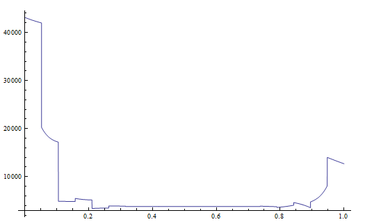
I then intend to use these functions in NDSolve, NIntegrate etc., therefore behaviour like above is too bad.
What parametric interpolation is better in this case?

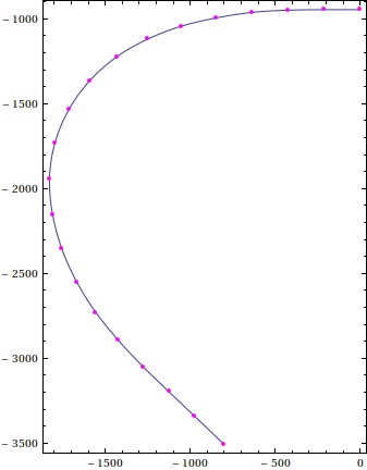

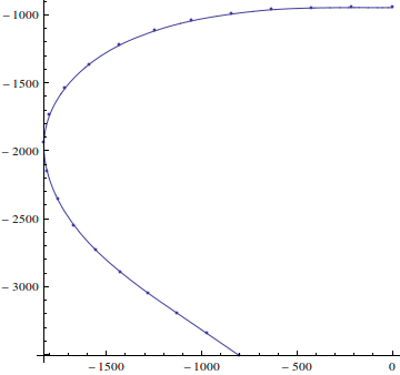
x1andy1? $\endgroup$xandyin mathematica.stackexchange.com/questions/19229/… $\endgroup$BSplineFunctionand then differentiating, you are taking a finite difference derivative sampled at whatever pointsPlotfeels like using. Try e.g.Plot[Norm[interp'[t]], {t, 0, 1}], which I think you will find much better. $\endgroup$