27
$\begingroup$

I have some problems in writing a module for spline smoothing. Actually, I have been trying for about two weeks. My listing is here:

SplSmooth[data_, knots_, lambda_, degree_] := 
  Module[{M, Knots, NKnots, NBasis, X, Dsq, a},
   M = Length@data;
   Knots = Flatten@{Table[1, {i, 1, degree}], knots,Table[M, {i,1,degree}]};
   NKnots = Length@Knots;
   NBasis = NKnots - degree - 1;
   X = Table[
     Evaluate @ BSplineBasis[{degree, Knots}, n, t] // N, {t, 1, M}, 
       {n, 0, NBasis - 1}];
   Dsq = Differences[X, 2];
   a=Inverse[Transpose[X].X + lambda*Transpose[Dsq].Dsq // N].Transpose[X].data // N;
   Return[X.a]
   ];

When I try to place a knot in every point in my data, numerical errors arise, such as:

Inverse::luc: Result for Inverse of badly conditioned matrix {{1.251,-0.1255,-0.251,0.0836667,0.0418333,0.,0.,0.,0.,0.,<<72>>},<<9>>,<<72>>} may contain significant numerical errors. >>

Obviously, the corresponding result is wrong (I can see it from the plot). It seems that the matrix to be inverted is ill-conditioned:

a = Inverse[Transpose[X].X + lambda*Transpose[Dsq].Dsq // N].Transpose[X].data // N;

but now comes the other problem. I use equidistant knots (let's say with 7 points distance) to overcome this problem. But then sometimes the algorithm works with:

Knots = Flatten @ {Table[1, {i, 1, degree}], knots, Table[M, {i, 1, degree}]};

and some other times works with

Knots = Flatten @ {Table[1, {i, 0, degree}], knots, Table[M, {i ,0, degree}]};

Now, I think that there is some kind of problem in BSplineBasis function.

Q: Can you spot the problem please? Or has anyone of you implemented a simillar function in the past with BSplineBasis function?

$\endgroup$
5
  • 7
    $\begingroup$ Always avoid calling Inverse when you can use LinearSolve. Solving a linear system is much faster and stabler than calculating an inverse. $\endgroup$
    – ssch
    Commented Sep 29, 2013 at 16:47
  • $\begingroup$ have you seen this? mathematica.stackexchange.com/… $\endgroup$ Commented Sep 29, 2013 at 17:00
  • $\begingroup$ Thank you very much ssch. The algorithm is more stable now. But I am still in doubt for the duplication of the first and the last point as knots. Anyway, you helped me a lot. $\endgroup$ Commented Sep 29, 2013 at 17:09
  • $\begingroup$ Actually the problem persists: LinearSolve::luc: "Result for ... of badly conditioned matrix may contain significant numerical errors. $\endgroup$ Commented Sep 29, 2013 at 17:21
  • $\begingroup$ Dear Belissarius thank you for your response. All these posts state that we must duplicate the external knots d times, where d is the degree of the spline. I know that fact, but why my second problem persists? Anyway, this correction seems to cure many instabilities, but not all: a = LinearSolve[ Transpose[X].X + lambda*Transpose[Dsq]. Dsq, Transpose[X].data, Method -> "Krylov"] // N; $\endgroup$ Commented Sep 29, 2013 at 17:51

4 Answers 4

31
$\begingroup$

I'm not sure if this addesses all of the issues you are having but here is an implementation I put together some time ago that allows us to use LinearModelFit and BSplineBasis to do spline regression.

The benefit of this approach is that all of the properties of FittedModel are immediately available to us. This allows for checking for fit, residual diagnostics etc.

SplineModel[data_, deg_, knots_] := 
  Block[{basis, allKnots}, 
   basis = 
    Array[\[FormalX]^# &, deg + 1, 0]~Join~
     Table[BSplineBasis[{deg, knots}, i, \[FormalX]], 
        {i, 0, Length[knots] - deg - 2}];

   LinearModelFit[data, basis, \[FormalX]]
];

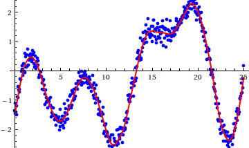
Lets generate some interesting data...

SeedRandom[249304]; data = 
 Table[{i, 
   RiemannSiegelZ[i] + Sin[i] + 
    RandomReal[NormalDistribution[0, .2]]}, {i, 0, 25, .05}];

And now we pick some knots and smooth the data using cubic splines.

knots = Range[0, 25, 1];
mod = SplineModel[data, 3, knots];

Show[ListPlot[data], Plot[mod[x], {x, 0, 25}, PlotStyle -> Directive[Red, Thick]]]

enter image description here

$\endgroup$
8
  • $\begingroup$ Thank you Andy. It seems that my only problem is the ill conditioning. I tried your approach and everything works fine, except from the absence of the smoothing parameter. Now, I think that in my approach, the term lambda*Transpose[Dsq].Dsq , witch is a faster alternative for roughness penalty, causes all the trouble. $\endgroup$ Commented Sep 30, 2013 at 20:53
  • $\begingroup$ Dear Andy, I've noticed that you are using as basis the terms 1,x,...x^degree and also the BSplineBasis function. Namely, you are using the B-splines and some functions of the truncated power basis. Is that approach correct? I am asking you because I've never seen this before. $\endgroup$ Commented Oct 1, 2013 at 7:21
  • 2
    $\begingroup$ What I have found is that adding these has the effect of minimizing edge effects. Feel free to remove these extra basis functions but also keep in mind that there is nothing inherently wrong with adding any basis functions we wish. $\endgroup$
    – Andy Ross
    Commented Oct 1, 2013 at 13:33
  • $\begingroup$ Hmm, where are n kmin and kmax used inside of SplineModel? $\endgroup$
    – Ajasja
    Commented Oct 16, 2014 at 12:27
  • $\begingroup$ @Ajasja oops, must have been copy/paste. I'm surprised no one caught that before now. I suspect the reason it was there in the first place was because my original code picked the knots automatically rather than using pre-set ones. $\endgroup$
    – Andy Ross
    Commented Oct 16, 2014 at 13:28
15
$\begingroup$

I have long been looking for a good implementation of cubic spline smoothing with adjustable roughness penalty parameter for Mathematica. Your module gave me enough hints to understand how to make this work in Mathematica, so I basically made a cubic spline smoothing code from your code with minor adjustments (about knots, a little bit about performance)

CubicSplSmooth[data_, lambda_] := 
  Module[{M, Knots, X, Dsq, a},
          M = Length @ data;
          Knots = Flatten @ { 1, 1, 1, Range @ M, M, M, M};
          X = Table[ Evaluate @ N @ BSplineBasis[{3, Knots}, n, t], 
                     {t, 1, M}, {n, 0, M + 1}];
          Dsq = Differences[X, 2];
          a = LinearSolve[ Transpose[X].X + lambda*Transpose[Dsq].Dsq, 
                           Transpose[X].data, Method -> "Multifrontal"];
          Return[X.a]
       ];

This is restricted to cubic degree, but can be generalized to arbitrary degree as in your example. Manipulate is a nice way to get a feeling for the performance by moving the slider around:

Manipulate[
    smoothdata = CubicSplSmooth[data, 10^lambda];
    Show[ ListPlot[ data, PlotRange -> {-5, 3}], 
          ListLinePlot[ smoothdata, Mesh -> All, PlotStyle -> Red]],
    {{lambda, 0}, -5, 5}]

The smoother behaves very naturally, yielding the original data for low (close to 0) values of lambda and a linear fit to data for extremely high ones.

If one compares this to the performance LabVIEW achieves with the Cubic Spline Fit VI, it is still slower, especially for large datasets. But the source of that is not accessible, I think. Anyway it works well up to now, but I think that performance can be surely improved.

$\endgroup$
5
  • 1
    $\begingroup$ Welcome to mathematica.SE and thanks for sharing :) $\endgroup$
    – ssch
    Commented Oct 27, 2013 at 13:56
  • $\begingroup$ The speed is the last thing that can bother us. We can use the Compile function, so the code will be transformed in the background into C code. And if Mathematica can reach gcc, then the result is really fast. $\endgroup$ Commented Oct 29, 2013 at 11:48
  • 1
    $\begingroup$ Also I've found that LeastSquares is a faster and more reliable command for matrix inversion problems, so it is preferred than LinearSolve for arbitrary data. $\endgroup$ Commented Oct 29, 2013 at 11:51
  • $\begingroup$ I think that the problem is the B-Spline functions themselves. They have the advantage to transform data in such way that all the math from least squares fitting can be applied without problem. But they still have problems with the stability and they aren't well documented. I am planning to use the "old school" approach from the book: Pollock, Handbook of Time Series Analysis, Signal Processing, and Dynamics. $\endgroup$ Commented Oct 29, 2013 at 12:57
  • $\begingroup$ @Tobi In the line: X = Table[ Evaluate @ N @ BSplineBasis[{3, Knots}, n, t],{t, 1, M}, {n, 0, M + 1}]; n & t have no definition. Was there a reason for these or is this a typo? $\endgroup$ Commented Jan 5, 2014 at 0:00
12
$\begingroup$

Here is a (simplified) implementation of Reinsch's smoothing spline, which is effectively equivalent to csaps() in MATLAB's Curve Fitting Toolbox. Fancier methods have come along since then (e.g. Wahba's cross-validation splines), but this old workhorse has still proved serviceable:

SmoothingSplineFunction[dat_?MatrixQ, p : (_?NumericQ | Automatic) : Automatic] :=
 Module[{n = Length[dat], pv = p, cc, dc, del, h, qg, qm, rh, tm, uv, xa, ya},
        {xa, ya} = Transpose[dat]; h = Differences[xa]; rh = 1/h; 
        del = Differences[ya] rh;
        qm = SparseArray[{Band[{1, 1}] -> Most[rh], 
                          Band[{1, 2}] -> -ListCorrelate[{1, 1}, rh], 
                          Band[{1, 3}] -> Rest[rh]}, {n - 2, n}];
        tm = SparseArray[{Band[{2, 1}] -> Most[Rest[h]],
                          Band[{1, 1}] -> ListCorrelate[{2, 2}, h],
                          Band[{1, 2}] -> Drop[h, -2]}, {n - 2, n - 2}];
        qg = qm.Transpose[qm];
        If[pv === Automatic, pv = 1/(1 + Tr[tm]/(6 Tr[qg]))];
        uv = LinearSolve[6 (1 - pv) qg + pv tm, Differences[del]];
        dc =
        ya - 6 (1 - pv) Differences[ArrayPad[Differences[ArrayPad[uv, 1]]/h, 1]];
        Interpolation[Transpose[{List /@ xa, dc, Append[Differences[dc]/h -
                                 h ListCorrelate[{2, 1}, ArrayPad[pv uv, 1]],
                                 pv Last[uv] Last[h] -
                                 (Subtract @@ Take[dc, -2])/Last[h]]}],
                      InterpolationOrder -> 3, Method -> "Hermite"]]

(It might be a bit confusing that the output is an InterpolatingFunction[] even though no interpolation is being done; it's just that I wanted to use the built-in facility for evaluating piecewise Hermite cubics.)

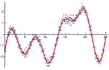
Let's use it on Andy's example:

BlockRandom[SeedRandom[249304]; 
            data = Table[{i, RiemannSiegelZ[i] + Sin[i] +
                          RandomVariate[NormalDistribution[0, .2]]},
                         {i, 0, 25, 0.05}]]
smth = SmoothingSplineFunction[data, 9/10];
Plot[smth[x], {x, 0, 25}, PlotStyle -> Directive[Thick, Red], 
     Prolog -> {Blue, AbsolutePointSize[5], Point[data]}]

Reinsch smoothing on Andy's example

There is an ad hoc element to choosing the "smoothing parameter" in the second argument, however. There have been a number of proposals on how to pick the best smoothing parameter, but I haven't gotten around to evaluating them, as I've mostly used smoothing splines only for looking at the approximate trend.

$\endgroup$
4
  • $\begingroup$ Would you be able to elaborate on how you would calculate the best smoothing parameter? I had an attempt to evaluate it but ended up with something very inefficient (see my question here mathematica.stackexchange.com/questions/219616/…). $\endgroup$ Commented Apr 21, 2020 at 11:39
  • $\begingroup$ @Daniele, I think Grace Wahba's papers have a procedure on that, but it has been a while since I delved into the relevant literature. $\endgroup$ Commented Apr 21, 2020 at 12:04
  • $\begingroup$ @JM I guess you are referring to tandfonline.com/doi/abs/10.1080/00401706.1979.10489751. However, I have difficulties in understanding your implementation of splines, so I cannot figure out how Wahba's X matrix (appearing in the abstract, which is the only thing I can read in that paper) is connected to any matrix you construct in your module. $\endgroup$ Commented Apr 22, 2020 at 9:10
  • $\begingroup$ "difficulties in understanding your implementation of splines" - it's mostly a straightforward translation of Reinsch's procedure; the matrix inside LinearSolve[] is exactly the same matrix that Reinsch solved in his ALGOL procedure through an embedded pentadiagonal solver. Here I use LinearSolve[] + SparseArray[] instead. If you want a deeper explanation of the code, you can always ask a new question. $\endgroup$ Commented Apr 22, 2020 at 11:55
7
$\begingroup$

Anton Antonov has implemented smoothing splines in his Quantile regression with B-splines package (direct link to the M-file). This post (duplicated in this thread) and this WTC2014 talk explain how can it be used. See also this post of mine for an example of use.

$\endgroup$

Your Answer

By clicking “Post Your Answer”, you agree to our terms of service and acknowledge you have read our privacy policy.

Not the answer you're looking for? Browse other questions tagged or ask your own question.