7
$\begingroup$

Bug introduced in 11.3 or earlier and persisting through 12.0.0 or later


While looking at https://mathematica.stackexchange.com/questions/192081/how-do-i-plot-a-divergence, I thought to suggest the following as a solution to the OP's problem (where potdistr is an InterpolatingFunction solution to a PDE returned by NDSolve):

VectorDensityPlot[
 Evaluate[Grad[potdistr[x, y], {x, y}]],
 {x, -0.01, 0.11}, {y, -0.005, 0.053}]

I surprised that it worked once and then failed on subsequent calls. It seems to be connected to InterpolatingFunction and values being set for x and y. Here is a minimal example:

field = {Interpolation[Range[4]^2/4][y], x};
VectorDensityPlot[field, {x, 1, 4}, {y, 1, 4}]

Subsequent calls generate a InterpolatingFunction::dmval extrapolation warning message and the vector field is constant.

The problem does not occur if field = {y^2/4, x} is used. It does not occur for VectorPlot, DensityPlot, ContourPlot, or Plot3D.

What's going on? Is it a bug? Is there a way to get it to work?

Additional info:

$Version
(*  "11.3.0 for Mac OS X x86 (64-bit) (January 22, 2018)"  *)

Filed as [CASE:4228039], confirmed by WRI.

$\endgroup$
1
  • $\begingroup$ I was fiddling with the same problem, and had odd results when attempting to do a StreamPlot of the gradient of potexpr. $\endgroup$
    – MikeY
    Commented Feb 24, 2019 at 15:55

2 Answers 2

7
$\begingroup$

What is happening is that x and y are being set equal to numeric values. (One might notice that the color for x and y changes from blue to black, but my eyes have trouble seeing that for single-letter variables.) For some reason, these values are outside the domain specified in the plot. I think this must be a bug and have reported it to WRI.

Clear[x, y]
{x, y}
field = {Interpolation[Range[4]^2/4][y], x};
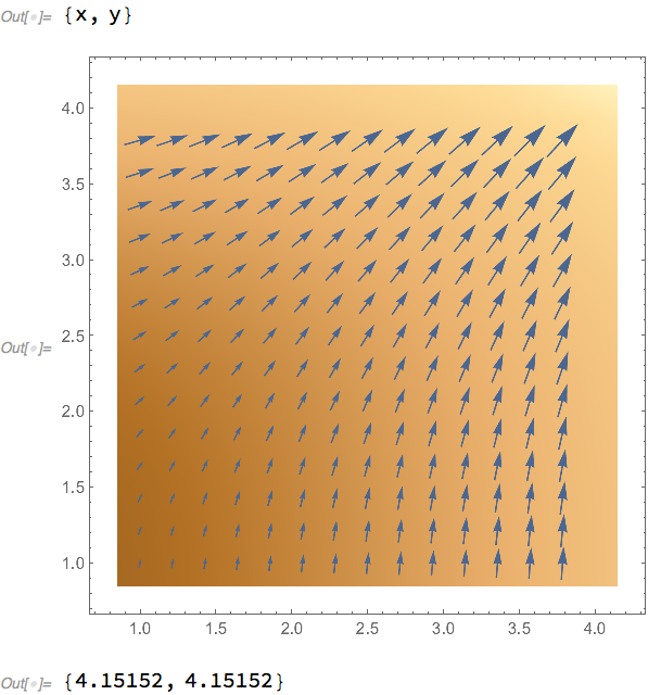
VectorDensityPlot[field, {x, 1, 4}, {y, 1, 4}]
{x, y}

enter image description here

One possible workaround is to clear the variables after plotting with Clear[x, y]. Another is to use Block:

Block[{x, y}, VectorDensityPlot[field, {x, 1, 4}, {y, 1, 4}]]

Further, it does not seem restricted only to InterpolatingFunction. The following has the same issue, and, further, VectorStyle is ignored:

Clear[x, y, ff]
{x, y}
ff[xx_, yy_] := {yy^2/4, xx};
VectorDensityPlot[ff[x, y], {x, 1, 4}, {y, 1, 4}, VectorStyle -> Red]
{x, y}
(*  output is the same as above, same coloring  *)

Pre-evaluating ff[x, y] gives the desired plot:

VectorDensityPlot[Evaluate@ff[x, y], {x, 1, 4}, {y, 1, 4}, VectorStyle -> Red]
$\endgroup$
2
$\begingroup$

This works...once you have potdistr, run this to get a Function

pdg = Evaluate[Grad[potdistr[#1, #2], {#1, #2}]] &

You can then run the plot function repeatedly, no problem, and go back and run previous statements (you couldn't when x, y were getting set).

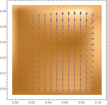
VectorDensityPlot[pdg[x,y], {x, 0, 0.1}, {y, 0, 0.05}]

enter image description here

You can also run this kludgy version, but it is slow.

VectorDensityPlot[Evaluate[Grad[potdistr[#1, #2], {#1, #2}]] &[x, y], 
                  {x, 0, 0.1}, {y, 0, 0.05}]

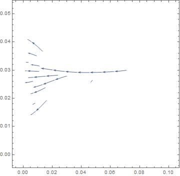
I was interested in the not very useful looking StreamPlot I was getting.

StreamPlot[pdg[x, y], {x, 0, 0.1}, {y, 0, 0.05}]

enter image description here

One thing I found odd is that if you look at the domain for potdistr versus the plot ranges people are using, there should be some extrapolation going on. Shouldn't we get warnings for that?

$\endgroup$
5
  • $\begingroup$ Can you explain why the first method works? It might be worth pointing out that VectorDensityPlot still sets x and y here, but this method gets around the trouble it causes in other methods. $\endgroup$
    – Michael E2
    Commented Feb 24, 2019 at 22:30
  • $\begingroup$ Frankly I’m not sure of the details, but it seems a best practice to define functions this way anyway. $\endgroup$
    – MikeY
    Commented Feb 25, 2019 at 1:04
  • $\begingroup$ On the one hand, it's because pdg does not depend on x or y. Instead, the gradient is computed by differentiating the function with respect to #1 and #2 (Slot[1] and Slot[2]) which are Protected. Mathematica allows this use of #1 and #2, which is convenient here. On the other hand, the x and y inside VectorDensityPlot[pdg[x, y],...] are effectively localized using Block. This means that any global values for x and y are temporarily cleared before the plot is calculated.... $\endgroup$
    – Michael E2
    Commented Feb 25, 2019 at 1:34
  • $\begingroup$ ....From these two reasons. your approach, while not preventing x and y from from being overwritten, solves the major problem of making the plot work. [Obviously, I knew the answer. I just thought the answer would be improved by an explanation, for others who are looking to understand Mathematica better. Since it's your answer, I was encouraging you to add such an explanation.] $\endgroup$
    – Michael E2
    Commented Feb 25, 2019 at 1:36
  • $\begingroup$ I like your explanation better. :) It's not always clear to me how an InterpolatingFunction's are set. $\endgroup$
    – MikeY
    Commented Feb 25, 2019 at 1:53

Your Answer

By clicking “Post Your Answer”, you agree to our terms of service and acknowledge you have read our privacy policy.

Not the answer you're looking for? Browse other questions tagged or ask your own question.