How to splice together several instances of InterpolatingFunction?

Question

I have a set of InterpolatingFunction returned by NDSolve which are valid over different (but overall continuous) domains. How do I splice them together into one single InterpolatingFunction over all the domains?

Piecewise seems to promising, but I can't manage to return the piecewise function from another function then use it later the same way as InterpolatingFunction.

I guess there is also the brute force way of generating a grid of points using the original set of InterpolatingFunction then interpolating points again, but that's very elaborate and CPU-consuming, not to mention potentially inaccurate if the interpolation grid is not chosen properly.

Thoughts?

---

Thanks to the answer from Mr. Wizard, this is the solution I ended up using:

JoinInterpolatingFunction[intervals_List, flist_List] := 
 Module[{getGrid},
  getGrid[f_InterpolatingFunction, min_?NumericQ, 
    max_?NumericQ] := {{min, f[min]}}~
     Join~(Transpose@{f["Grid"] // Flatten, f["ValuesOnGrid"]} // 
       Select[#, (min < #[[1]] < max) &] & )~Join~{{max, f[max]}} // N;
  Interpolation[
   Table[getGrid[flist[[i]], intervals[[i]], intervals[[i + 1]]], {i, 
       Length@flist}] // Flatten[#, 1] & // 
    DeleteDuplicates[#, (#1[[1]] == #2[[1]]) &] &, 
   InterpolationOrder -> 2]]

JoinInterpolatingFunction[{I1,I2,..,In},{func1,func2,...func(n-1)}] gives an InterpolatingFunction that takes values of func1 between [I1,I2], func2 between (I2,I3], ... func(n-1) between (I(n-1),In].

Answer 1

Update: information below updated with values from version 10.0.0

I expect that if the InterpolationOrder is the same between functions it should be possible to merge them into one. If not Piecewise may be the best you can do.

This is an incomplete answer but hopefully a useful signpost that may lead you to a solution. You can get the constituent parts (or at least their related forms) using the little-known "Methods" syntax, which is akin to the "Properties" of SparseArray if you have seen that before.

Here is a list of the "Methods":

f1 = Interpolation @ Table[{i, Sin[i]}, {i, 0, Pi, 0.1}];
f1["Methods"]

{"Coordinates", "DerivativeOrder", "Domain", "ElementMesh", "Evaluate", "Grid",
"InterpolationMethod", "InterpolationOrder", "MethodInformation", "Methods",
"OutputDimensions", "Periodicity", "PlottableQ", "Properties", "QuantityUnits",
"ValuesOnGrid"}

Here are the internal usage messages:

f1["MethodInformation"@#] & ~Scan~ f1["Methods"]

• InterpolatingFunction[domain, data]@Coordinates[] returns the grid coordinates in each dimension.

• InterpolatingFunction[domain, data]@DerivativeOrder[] returns what derivative of the interpolated function will be computed upon evaluation.

• InterpolatingFunction[domain, data]@Domain[] returns the domain of the InterpolatingFunction.

• InterpolatingFunction[domain, data]@ElementMesh[] returns the element mesh if one is present.

• InterpolatingFunction[domain, data]@Evaluate[arg] evaluates the InterpolatingFunction at the argument arg.

• InterpolatingFunction[domain, data]@Grid[] gives the grid of points where the interpolated data is defined.

• InterpolatingFunction[domain, data]@InterpolationMethod[] returns the method used for interpolation.

• InterpolatingFunction[domain, data]@InterpolationOrder[] returns the degree of polynomials used for computing interpolated values.

• InterpolatingFunction[domain, data]@MethodInformation[method] gives information about a particular method.

• InterpolatingFunction[domain, data]@Methods[pat] gives the list of methods matching the string pattern pat.

• InterpolatingFunction[domain, data]@OutputDimensions[] returns the output dimensions of the interpolating function.

• InterpolatingFunction[domain, data]@Periodicity[] returns whether the interpolating function is periodic in the respective dimensions.

• InterpolatingFunction[domain, data]@PlottableQ[] returns whether the interpolating function is plottable or not.

• InterpolatingFunction[domain, data]@Properties gives the list of possible properties.

• InterpolatingFunction[domain, data]@QuantityUnits[] returns the quantity units associated with abscissa and ordinates.

• InterpolatingFunction[domain, data]@ValuesOnGrid[] gives the function values at each grid point. In some cases, this may be faster than evaluating at each of the grid points.

Here is the actual output when applying these "Methods" to the example InterpolatingFunction above:

Print /@ f1 /@ {"Coordinates", "DerivativeOrder", "Domain", "ElementMesh", Evaluate[], "Grid", 
   "InterpolationMethod", "InterpolationOrder", "Methods", "OutputDimensions", 
   "Periodicity", "PlottableQ", "Properties", "QuantityUnits", "ValuesOnGrid"};

{{0.,0.1,0.2,0.3,0.4,0.5,0.6,0.7,0.8,0.9,1.,1.1,1.2,1.3,1.4,1.5,1.6,1.7,1.8,1.9,2.,2.1,2.2,2.3,2.4,2.5,2.6,2.7,2.8,2.9,3.,3.1}}

0

{{0.,3.1}}

None

{{0.},{0.1},{0.2},{0.3},{0.4},{0.5},{0.6},{0.7},{0.8},{0.9},{1.},{1.1},{1.2},{1.3},{1.4},{1.5},{1.6},{1.7},{1.8},{1.9},{2.},{2.1},{2.2},{2.3},{2.4},{2.5},{2.6},{2.7},{2.8},{2.9},{3.},{3.1}}

Hermite

{3}

{Coordinates,DerivativeOrder,Domain,ElementMesh,Evaluate,Grid,InterpolationMethod,InterpolationOrder,MethodInformation,Methods,OutputDimensions,Periodicity,PlottableQ,Properties,QuantityUnits,ValuesOnGrid}

{}

{False}

True

{Properties}

{None,None}

{0.,0.0998334,0.198669,0.29552,0.389418,0.479426,0.564642,0.644218,0.717356,0.783327,0.841471,0.891207,0.932039,0.963558,0.98545,0.997495,0.999574,0.991665,0.973848,0.9463,0.909297,0.863209,0.808496,0.745705,0.675463,0.598472,0.515501,0.42738,0.334988,0.239249,0.14112,0.0415807}

Answer 2

Chaining extrapolation handlers

We can chain together the extrapolation handlers. It will overwrite any existing extrapolation handler except in the last interpolating function; however, that seems consistent with the goal of splicing together interpolating functions.

We can find the position of the extrapolation handler this way (see also What's inside InterpolatingFunction[{{1., 4.}}, <>]? for more on the structure of InterpolatingFunction):

Block[{f = Unique["ExtrapolationHandler"]}, 
  First@Position[Interpolation[Range[4], "ExtrapolationHandler" -> {f}], f]]
(*  {2, 10}  *)

Then we can fold together the interpolating function thus:

With[{extrapHandlerPos = Block[{f = Unique["ExtrapolationHandler"]}, 
    First@Position[Interpolation[Range[4], "ExtrapolationHandler" -> {f}], f]]},
 interpolationJoin[ifns__] := 
   Fold[ReplacePart[#2, extrapHandlerPos -> #1] &, Reverse@Flatten[{ifns}]]]

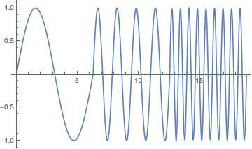
Test case:

ifns = Table[
  Interpolation@Table[{x + 2 Pi i, Sin[i^2 x]}, {x, -2 Pi, 0, 2 Pi/60}], {i, 3}];
if = interpolationJoin[ifns];

Plot[if[x], {x, 0, 6 Pi}]

---

V10: Joining multivariable interpolating functions

Using Piecewise with a Cuboid region for each domain, we can piece together functions of any number of variables (as long as the number of variables is the same).

Clear[interpolationJoin];
interpolationJoin[ifns__, vars_] /; 
    Apply[Equal, Length[#["Domain"]] & /@ Flatten[{ifns}]] :=
  Piecewise @@
    {{# @@ Flatten[{vars}], Flatten[{vars}] ∈ Cuboid @@ Transpose[#["Domain"]]} & /@
       Flatten[{ifns}]}

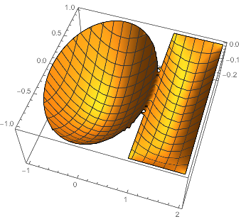
Test case:

ifns2d = {NDSolveValue[
    {Laplacian[u[x, y], {x, y}] == 1, DirichletCondition[u[x, y] == 0, True]}, 
    u, {x, y} ∈ Disk[], 
    "ExtrapolationHandler" -> {Indeterminate &, "WarningMessage" -> False}],
   NDSolveValue[
    {Laplacian[u[x, y], {x, y}] == 1, DirichletCondition[u[x, y] == 0, True]}, 
    u, {x, y} ∈ Cuboid[{1, -1}, {2, 1}], 
    "ExtrapolationHandler" -> {Indeterminate &, "WarningMessage" -> False}]};

if2 = interpolationJoin[ifns2d, {x, y}];

Plot3D[if2, {x, -1, 2}, {y, -1, 1}]

Note: For a more sophisticated approach, one could test for an ElementMesh domain in each interpolating function and use that instead of a cuboid, when an ElementMesh is present.

Answer 3

It could well be that one of the other suggestions will lead you to what you'll be using in the end. I think you should still know about the most straightforward way to create a combination of interpolating functions using Piecewise and a pure function:

ipf1 = Interpolation[Table[{x, Sin[x]}, {x, 0, 1, 0.1}]]
ipf2 = Interpolation[Table[{x, Sin[x]}, {x, 1, Pi, 0.1}]]
ipfCombined = Function[Piecewise[{{ipf1[#], # <= 1}, {ipf2[#], # > 1}}]]

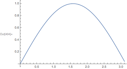
the result can almost everywhere be used just like an InterpolatingFunction:

Plot[ipfCombined[x], {x, 0, Pi}]
Integrate[ipfCombined[x], {x, 0, Pi}]

(if you want to show a continuous plot you can add the option Exclusions -> None)

Answer 4

If you explicitly want to join the list of coordinates for e.g. two univariate InterpolatingFunctions (i.e. not opting for Piecewise), you can use the InterpolatingFunctionAnatomy package, that allows extraction of coordinates and grid points of ip.functions:

Needs["DifferentialEquations`InterpolatingFunctionAnatomy`"];

Options[joinInterpolation] = Options[Interpolation];
joinInterpolation[int : {__InterpolatingFunction}, opts___] := Module[{coord, vals},
   coord = Join @@ (First@InterpolatingFunctionCoordinates@# & /@ int);
   vals = Join @@ (InterpolatingFunctionValuesOnGrid /@ int);
   Interpolation[MapThread[List, {coord, vals}], opts]
   ];

Test the function:

ipf1 = Interpolation[Table[{x, Sin[x]}, {x, 0, Pi, 0.1}]];
ipf2 = Interpolation[Table[{x, Sin[x]}, {x, Pi, 2 Pi, 0.1}]];
joined = joinInterpolation[{ipf1, ipf2}];

Row@{Plot[ipf1[t], {t, 0, Pi}],
     Plot[ipf2[t], {t, Pi, 2 Pi}],
     Plot[joined[t], {t, 0, 2 Pi}]
    }

Answer 5

You could use NDSolve to piece together the interpolating functions. For example:

ipf1 = Interpolation[Table[{x, Sin[x]}, {x, 0, 1, 0.1}]];
ipf2 = Interpolation[Table[{x, Sin[x]}, {x, 1, Pi, 0.1}]];

if = NDSolveValue[
    {y'[x] == Piecewise[{{ipf1'[x], x<1}}, ipf2'[x]], y[0] == ipf1[0]},
    y,
    {x, 0, 3.1}
];
if //OutputForm

InterpolatingFunction[{{0., 3.1}}, <>]

Visualization:

Plot[if[x], {x, 0, 3.1}]

Answer 6

Nothing much to add here...this is just a slight modification to István's answer where the call to Needs has been removed in favour of Mr. Wizard's undocumented trick. The calling syntax is slightly different, and I also call DeleteDuplitacesBy to avoid the Interpolation warning about multiple points at a single coordinate.

Options[JoinInterpolatingFunction] = Options[Interpolation];
JoinInterpolatingFunction[int__InterpolatingFunction, opts:OptionsPattern[]] := Module[{data},
    data = {Join @@ (First[#["Coordinates"]] & /@ {int}), Join @@ (#["ValuesOnGrid"] & /@ {int})}\[Transpose];
    data = DeleteDuplicatesBy[data,First];
    Interpolation[data, opts]
];

Test the function:

ipf1 = Interpolation[Table[{x, Sin[x]}, {x, 0, Pi, Pi/16}]];
ipf2 = Interpolation[Table[{x, Sin[x]}, {x, Pi, 2 Pi, Pi/16}]];
joined = JoinInterpolatingFunction[ipf1, ipf2];

Row@{Plot[ipf1[t], {t, 0, Pi}], Plot[ipf2[t], {t, Pi, 2 Pi}], 
  Plot[joined[t], {t, 0, 2 Pi}]}