39
$\begingroup$

I've used Interpolation[] to generate an InterpolatingFunction object from a list of integers.

f = Interpolation[{2, 5, 9, 15, 22, 33, 50, 70, 100, 145, 200, 280, 375, 495, 635, 800,
                   1000, 1300, 1600, 2000, 2450, 3050, 3750, 4600, 5650, 6950}]

I'm using that to generate values like f[27], f[28], ...

Is there any way to print or show the function used by Mathematica that produced the result of f[27]?

$\endgroup$
11
  • 1
    $\begingroup$ You can view the internal parts of an InterpolatingFunction using "Methods" as I outlined here: (19042) however that only shows the data that is used and the kind of interpolation, not the actual function itself. You might find value in InterpolatingPolynomial, though it is not the same as Interpolation. $\endgroup$
    – Mr.Wizard
    Commented Sep 17, 2014 at 19:33
  • 6
    $\begingroup$ See Properties and Relations for an example; see also Some Notes on Internal Implementation. $\endgroup$
    – Michael E2
    Commented Sep 17, 2014 at 19:34
  • $\begingroup$ I am pretty sure that Mathematica uses interpolating polynomials, using Neville's algorithm. It is easy to implement this yourself and see if you get the same value. $\endgroup$
    – Igor Rivin
    Commented Sep 17, 2014 at 23:57
  • 2
    $\begingroup$ Maybe you want InterpolatingPolynomial instead of Interpolation. $\endgroup$
    – Szabolcs
    Commented Oct 12, 2017 at 13:07
  • 1
    $\begingroup$ @Szabolcs if I'm reading this right, certainly not. That one gives a polynomial of arbitrarily high degree which is probably not that useful. $\endgroup$
    – LLlAMnYP
    Commented Oct 12, 2017 at 13:23

7 Answers 7

33
$\begingroup$

Here is the example from the documentation adapted for the OP's data:

data = MapIndexed[
   Flatten[{#2, #1}] &,
   {2, 5, 9, 15, 22, 33, 50, 70, 100, 145, 200, 280, 375, 495, 635, 800,
    1000, 1300, 1600, 2000, 2450, 3050, 3750, 4600, 5650, 6950}];
f = Interpolation@data
(* InterpolatingFunction[{{1, 26}}, <>] *)
pwf = Piecewise[
     Map[{InterpolatingPolynomial[#, x], x < #[[3, 1]]} &, Most[#]], 
     InterpolatingPolynomial[Last@#, x]] &@Partition[data, 4, 1];

Here is a comparison of the piecewise interpolating polynomials and the interpolating function:

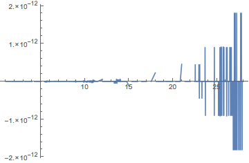
Plot[f[x] - pwf, {x, 1, 28}, PlotRange -> All]

Mathematica graphics

The values of f[27] and f[28] are beyond the domain, which is 1 <= x <= 26, and extrapolation is used. The formula for extrapolation is given by the last InterpolatingPolynomial in pwf:

Last@pwf
(* 3750 + (850 + (100 + 25/3 (-25 + x)) (-24 + x)) (-23 + x) *)

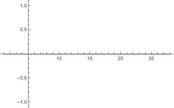
In response to a comment: The error in the plot has to do with round-off error. Apparently the calculation done by InterpolatingFunction, while algebraically equivalent, is not numerically identical. The error was greatest above in the domain 26 < x < 28 where extrapolation is performed. With arbitrary precision, the error is zero, as shown below.

Plot[f[x] - pwf, {x, 1, 28}, PlotRange -> All, 
 WorkingPrecision -> $MachinePrecision, Exclusions -> None, PlotStyle -> Red]

Mathematica graphics

$\endgroup$
8
  • $\begingroup$ (+1) The data in your answer should be defined as simple 1D list in order your code to work properly. How do you explain relatively large differences (1*10^-12) between your implementation and the built-in? $\endgroup$ Commented Sep 18, 2014 at 6:36
  • $\begingroup$ @AlexeyPopkov Thanks. See the update for the error explanation. (I copied the wrong code by mistake. It should work now.) $\endgroup$
    – Michael E2
    Commented Sep 18, 2014 at 11:16
  • 1
    $\begingroup$ Thanks, it is clear now. I would add that plotting relative error would be more correct and it clearly shows that the relative error is of expected magnitude of lesser than 10^-15: Plot[(f[x] - pwf)/pwf, {x, 1, 28}, PlotRange -> All]. $\endgroup$ Commented Sep 18, 2014 at 11:32
  • 1
    $\begingroup$ @LLlAMnYP There is no example in the linked dupe, but, yes, the old code assumed the abscissae were successive integers. Fixed now, I think. Let me know if it doesn't work for you. It won't work on all InterpolatingFunction methods, I think, just this type. $\endgroup$
    – Michael E2
    Commented Oct 12, 2017 at 15:39
  • 1
    $\begingroup$ @LLlAMnYP The method above does work on unequally spaced points, but not if the spacing varies wildly. It appears that InterpolatingFunction automatically splits data at points that are too close (I can get it to match if there aren't too many too-close points in a row). Or maybe it adapts the order locally. I don't know the criterion used. It is perhaps if the slope is too great in some relative sense. The result of InterpolatingFunction seems worse than the piecewise one in the example I got from your (random) code. Interesting -- didn't know it did such complicated things. $\endgroup$
    – Michael E2
    Commented Oct 13, 2017 at 11:49
24
$\begingroup$

There is no documented built-in way to convert the InterpolatingFunction object into explicit Piecewise form (thanks to @MichaelE2 for the link!). So the only possibility to get an explicit interpolating function is to re-implement the built-in Interpolation in the high-level Mathematica language. I have already done this for the built-in "Spline" method with InterpolationOrder -> 2 (quadratic spline interpolation with splicing points in the middle of adjacent interpolation points). Spline interpolation in general gives much better results than the default "Hermite" method.

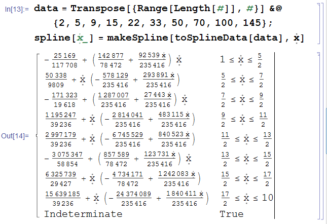
You can use my implementation of quadric spline interpolation in Mathematica to produce an explicit Piecewise function interpolating your data (as opposed to the built-in, it supports arbitrary precision!):

data = Transpose[{Range[Length[#]], #}] &@{2, 5, 9, 15, 22, 33, 50, 70, 100, 145};
spline[\[FormalX]_] = makeSpline[toSplineData[data], \[FormalX]]

screenshot

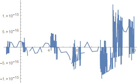
Here is a comparison with the original data and with the built-in Interpolation:

Table[data[[x, 2]] - spline[x], {x, 10}]
f = Interpolation[data, Method -> "Spline", InterpolationOrder -> 2];
Table[f[x] - spline[x], {x, 10}]
Plot[(f[x] - spline[x])/spline[x], {x, 1, 10}, PlotRange -> All]
{0, 0, 0, 0, 0, 0, 0, 0, 0, 0}
{0., 0., 0., 1.77636*10^-15, 0., 0., 0., 0., 0., 0.}

plot

$\endgroup$
4
  • $\begingroup$ Is it equivalent to what Mma implements for Interpolation[pts]? $\endgroup$ Commented Sep 18, 2014 at 1:24
  • $\begingroup$ @belisarius It is equivalent to Interpolation[pts, Method -> "Spline", InterpolationOrder -> 2] with the only difference that my implementation supports arbitrary precision while the current Mathematica's built-in for "Spline" allows only MachinePrecision. $\endgroup$ Commented Sep 18, 2014 at 1:28
  • $\begingroup$ I answered the same question where you wrote that answer, but I think the OP is asking another specific thing here about the InterpolatingFunctionoject $\endgroup$ Commented Sep 18, 2014 at 1:31
  • $\begingroup$ You know that there is no documented built-in way to convert InterpolatingFunction into explicit Piecewise form. I am sure that there is no undocumented way too because (at least "Hermite" method) is written in C, not in the high-level Mathematica language. So the only possibility to answer the question is to provide a high-level (re)implementation of the Interpolation. $\endgroup$ Commented Sep 18, 2014 at 1:38
18
+100
$\begingroup$

In M11+ you can use the "GetPolynomial" method of an interpolating function to obtain the corresponding piecewise expression (but only when using the default "Hermite" method):

InterpolationToPiecewise[if_, x_] := Module[{main, default, grid},
    grid = if["Grid"];
    Piecewise[
        {if @ "GetPolynomial"[#, x-#], x < First @ #}& /@ grid[[2 ;; -2]],
        if @ "GetPolynomial"[#, x-#]& @ grid[[-1]]
    ]
] /; if["InterpolationMethod"] == "Hermite"

For your example:

f = Interpolation[{2, 5, 9, 15, 22, 33, 50, 70, 100, 145, 200, 280, 375, 495, 635, 800,
               1000, 1300, 1600, 2000, 2450, 3050, 3750, 4600, 5650, 6950}];
pw = InterpolationToPiecewise[f, x];
pw //TeXForm

$\begin{cases} \left(\left(\frac{x-3}{6}+\frac{1}{2}\right) (x-1)+3\right) (x-2)+5 & x<2 \\ \left(\left(\frac{x-4}{6}+1\right) (x-2)+4\right) (x-3)+9 & x<3 \\ \left(\left(\frac{5-x}{6}+\frac{1}{2}\right) (x-3)+6\right) (x-4)+15 & x<4 \\ \left(\left(\frac{x-6}{2}+2\right) (x-4)+7\right) (x-5)+22 & x<5 \\ \left(\left(\frac{x-7}{3}+3\right) (x-5)+11\right) (x-6)+33 & x<6 \\ \left(\left(\frac{8-x}{2}+\frac{3}{2}\right) (x-6)+17\right) (x-7)+50 & x<7 \\ \left(\left(\frac{7 (x-9)}{6}+5\right) (x-7)+20\right) (x-8)+70 & x<8 \\ \left(\left(\frac{5 (x-10)}{6}+\frac{15}{2}\right) (x-8)+30\right) (x-9)+100 & x<9 \\ \left(\left(5-\frac{5 (x-11)}{6}\right) (x-9)+45\right) (x-10)+145 & x<10 \\ \left(\left(\frac{5 (x-12)}{2}+\frac{25}{2}\right) (x-10)+55\right) (x-11)+200 & x<11 \\ \left(\left(\frac{15}{2}-\frac{5 (x-13)}{3}\right) (x-11)+80\right) (x-12)+280 & x<12 \\ \left(\left(\frac{5 (x-14)}{3}+\frac{25}{2}\right) (x-12)+95\right) (x-13)+375 & x<13 \\ \left(\left(10-\frac{5 (x-15)}{6}\right) (x-13)+120\right) (x-14)+495 & x<14 \\ \left(\left(\frac{5 (x-16)}{6}+\frac{25}{2}\right) (x-14)+140\right) (x-15)+635 & x<15 \\ \left(\left(\frac{5 (x-17)}{3}+\frac{35}{2}\right) (x-15)+165\right) (x-16)+800 & x<16 \\ \left(\left(\frac{65 (x-18)}{6}+50\right) (x-16)+200\right) (x-17)+1000 & x<17 \\ \left(300-\frac{50}{3} (x-19) (x-17)\right) (x-18)+1300 & x<18 \\ \left(\left(\frac{50 (x-20)}{3}+50\right) (x-18)+300\right) (x-19)+1600 & x<19 \\ \left(\left(25-\frac{25 (x-21)}{3}\right) (x-19)+400\right) (x-20)+2000 & x<20 \\ \left(\left(\frac{50 (x-22)}{3}+75\right) (x-20)+450\right) (x-21)+2450 & x<21 \\ \left(\left(50-\frac{25 (x-23)}{3}\right) (x-21)+600\right) (x-22)+3050 & x<22 \\ \left(\left(\frac{25 (x-24)}{3}+75\right) (x-22)+700\right) (x-23)+3750 & x<23 \\ \left(\left(\frac{25 (x-25)}{3}+100\right) (x-23)+850\right) (x-24)+4600 & x<24 \\ \left(\left(\frac{25 (x-26)}{3}+125\right) (x-24)+1050\right) (x-25)+5650 & x<25 \\ \left(\left(\frac{25 (x-24)}{3}+125\right) (x-25)+1300\right) (x-26)+6950 & \text{True} \end{cases}$

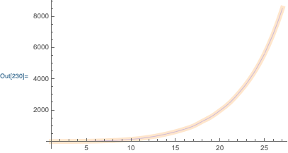
Visualization:

Plot[
    {f[x], pw},
    {x, 1, 27},
    PlotStyle->{Directive[Thickness[.02], LightOrange], Directive[Thin, Blue]}
]

enter image description here

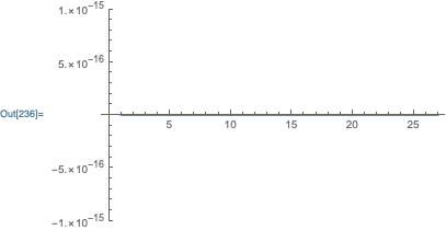
The error is negligible:

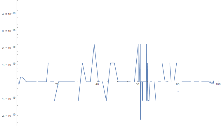
Plot[f[x]-pw, {x, 1, 27}, PlotRange->{-10^-15, 10^-15}]

enter image description here

$\endgroup$
3
  • $\begingroup$ points = {{1, 4}, {2, 7}, {3, 2}, {4, 8}, {5, 9}};InterpolationToPiecewise[if_, x_] := Module[{main, default, grid}, grid = if["Grid"]; Piecewise[{if@"GetPolynomial"[#, x - #], x < First@#} & /@ grid[[2 ;; -2]], if@"GetPolynomial"[#, x - #] &@grid[[-1]]]] /; if["InterpolationMethod"] == "Hermite" f2 = Interpolation[points, InterpolationOrder -> 2, Method -> "Spline"]; pw = InterpolationToPiecewise[f2, x] But this case with parameters can not output the desired results. $\endgroup$ Commented Jan 29, 2020 at 5:46
  • 6
    $\begingroup$ @Please, because you added Method -> "Spline" when Carl said that this function is only intended for Method -> "Hermite". $\endgroup$ Commented Jan 29, 2020 at 6:16
  • 1
    $\begingroup$ I wonder if x < First @ # should be x <= First @ #. Then with an interpolating function of InterpolationOrder -> 2, the derivatives at the nodes of the interpolating function and the piecewise function with differentiated polynomials agree. It may seem a moot point, since the true derivative is undefined at the nodes in general. See this example for a case where there is computational disagreement: pastebin.com/Mcd8kCwz . Ref: the commentary here. $\endgroup$
    – Michael E2
    Commented Jun 27, 2023 at 16:14
13
$\begingroup$

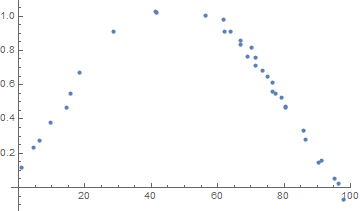
You could use Series. What's necessary is to know which abscissa values were used for the interpolation. Let's generate some fake data.

xVals = RandomReal[{0, 100}, 35] // Sort;
yVals = Sin[xVals/30] + RandomReal[.1, 35];
ListPlot[{xVals, yVals}\[Transpose]]

enter image description here

Create the interpolation:

iPol = Interpolation[{xVals, yVals}\[Transpose]]

Get the Series expansion at some point:

Series[iPol[x], {x, xVals[[5]], 4}]
0.469053+0.0487866 (x-14.3715)+0.011059 (x-14.3715)^2+0.00100578 (x-14.3715)^3+O[x-14.3715]^5

Note that there is no 4th order term (as expected, since default interpolation order is 3).

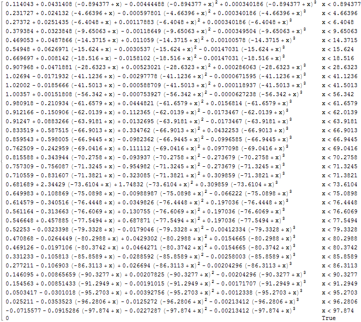
Let's generate a piecewise function:

pW[x_] = Piecewise[
  Table[{Normal@Series[iPol[x], {x, x0, 3}], x < x0}, {x0, xVals}]]

enter image description here

Test it out:

Plot[pW[x] - iPol[x], {x, xVals[[1]], xVals[[-1]]} PlotRange->Full]

enter image description here

Looks like (almost) machine precision to me

$\endgroup$
2
  • $\begingroup$ Thanks for your answer. That's indeed a uniform way to find the explicit representation. $\endgroup$
    – user52830
    Commented Oct 12, 2017 at 13:22
  • $\begingroup$ @user52830 You're welcome. Barring edge cases, if you happen to have just the InterpolatingFunction object, you can modify my Table statement as Table[..., {x0, iPol[[3,1]]}] since iPol[[3,1]] === xVals $\endgroup$
    – LLlAMnYP
    Commented Oct 12, 2017 at 13:26
12
$\begingroup$

Here is a (mostly) general routine that (tries to) convert a one-dimensional InterpolatingFunction[] into an equivalent Piecewise[] function:

convertToPiecewise::umet = "Unknown interpolation method `1`.";
SetAttributes[convertToPiecewise, Listable];

convertToPiecewise[iF_InterpolatingFunction, x_,
                   OptionsPattern[{"Extrapolation" -> False,
                                   InterpolationOrder -> Automatic}]] := 
       Module[{bf, extQ, imet, kp, makePP, met, nodes, perQ, pieces, pts, vand, xt},
              Switch[met = iF["InterpolationMethod"],
                     "Hermite" | "Chebyshev",
                     pts = Transpose[{Flatten[iF["Grid"]], iF["ValuesOnGrid"]}],
                     "BSpline",
                     bf = First[Cases[iF, _BSplineFunction, ∞]];
                     pts = {#, bf[#]} & /@ Union[First[bf["Knots"]]],
                     _,
                     Message[convertToPiecewise::umet, met]; Return[$Failed, Module]];
              kp = OptionValue[InterpolationOrder];
              If[kp === Automatic,
                 (* repeated differentiation to determine maximal order *)
                 kp = If[met =!= "BSpline",
                         First[NestWhile[Derivative[1],
                                         Derivative[First[iF["InterpolationOrder"]] +
                                                    1][iF],
                                         (Norm[#["ValuesOnGrid"], ∞] > 0) &]
                               ["DerivativeOrder"]] - 1,
                 kp = First[bf["Degree"]]]];
              If[kp > 0, (* normal case *)
                 (* use equispaced nodes in the exact case, and Chebyshev otherwise *)
                 nodes = Range[kp - 1]/kp;
                 If[MatrixQ[pts, InexactNumberQ],
                    nodes = N[Haversine[π nodes], Precision[pts]]];
                 vand = LinearAlgebra`Private`VandermondeSolve[##, Transpose -> True] &;
                 makePP[{{x1_, y1_}, {x2_, y2_}}] := Module[{h = x2 - x1, ip},
                     ip = Transpose[Join[{{x1 - x1, y1}},
                                         {#, iF[x1 + #]} & /@ (h nodes), {{h, y2}}]];
                     (* solve for interpolating polynomial coefficients *)
                     {Fold[(#1 (xt - x1) + #2) &, Reverse[vand @@ ip]], x1 <= xt <= x2}];
                 pieces = makePP /@ Partition[pts, 2, 1],
                 (* zero-order interpolation *)
                 pieces = Transpose[{Rest[pts[[All, -1]]],
                                     #1 <= xt <= #2 & @@@
                                     Partition[pts[[All, 1]], 2, 1]}]];
              perQ = TrueQ[First[iF["Periodicity"]]];
              If[! perQ, extQ = OptionValue["Extrapolation"];
                 If[! ListQ[extQ], extQ = {extQ, extQ}]; extQ = TrueQ /@ extQ;
                 If[extQ[[1]], pieces[[1, 2]] = Delete[pieces[[1, 2]], 1]];
                 If[extQ[[2]], pieces[[-1, 2]] = Delete[pieces[[-1, 2]], 3]]];
                 Piecewise[pieces /. xt ->
                           If[! perQ, x, Mod[x, #2 - #1, #1] & @@ First[iF["Domain"]]]]]

(N.B. replace LinearAlgebra`Private`VandermondeSolve[] with LinearAlgebra`VandermondeSolve[] when using the function in versions before 11.2.)

It should work for InterpolatingFunction[] objects that come from Interpolation[], ListInterpolation[], or FunctionInterpolation[]. It mostly works for InterpolatingFunction[] objects from NDSolve[], but may fail in some cases. (If you find an example, please tell me!)

Some examples:

if1 = Interpolation[{1, 3, 5, 2, 1}, InterpolationOrder -> 1];

Here, we tell convertToPiecewise[] to use the rightmost piece for extrapolation to the right:

convertToPiecewise[if1, x, "Extrapolation" -> {False, True}]

$$\begin{cases} 2 (x-1)+1 & 1\leq x\leq 2 \\ 2 (x-2)+3 & 2\leq x\leq 3 \\ 5-3 (x-3) & 3\leq x\leq 4 \\ 6-x & 4\leq x \\ 0 & \mathtt{True} \end{cases}$$

Convert an InterpolatingFunction[] with irregular spacing:

if2 = Interpolation[{{0, 0}, {0.1, .3}, {0.5, .6}, {1, -.2}, {2, 3}}, Method -> "Spline"];

pw2[x_] = convertToPiecewise[if2, x];

Plot[if4[x] - pw4[x], {x, 0, 2}, PlotRange -> All]
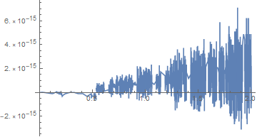
spline interpolant error

Convert the result of NDSolve[]:

if3 = NDSolveValue[{g'[x] == Sin[2 x] - g[x], g[0] == 1}, g, {x, 0, 6}];

pw3[x_] = convertToPiecewise[if3, x];

Plot[if3[x] - pw3[x], {x, 0, 6}, PlotRange -> All]
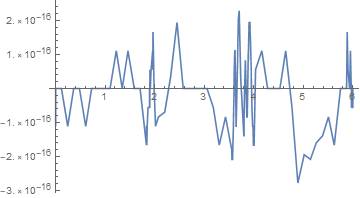
error of interpolant from NDSolve

Another NDSolve[] example. The previous version of the routine was unable to handle this.

if4 = NDSolveValue[{y''[t] == 10 (1 - y[t]^2) y[t] - y[t], y[0] == 2, y'[0] == 0},
                   y, {t, 0, 6}, Method -> "StiffnessSwitching"];

pw4[x_] = convertToPiecewise[if4, x];

Plot[if4[x] - pw4[x], {x, 0, 6}, PlotRange -> All]
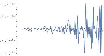
error of interpolant from NDSolve, second order

$\endgroup$
7
  • 1
    $\begingroup$ I seem to have to use LinearAlgebra`Private`VandermondeSolve; I can't get LinearAlgebra`VandermondeSolve to evaluate on anything. (V11.2, Mac). $\endgroup$
    – Michael E2
    Commented Mar 24, 2018 at 22:28
  • 1
    $\begingroup$ Ah, you're right, I was doing this in 11.1. I'll add a note... $\endgroup$ Commented Mar 25, 2018 at 1:02
  • $\begingroup$ Within Mathematica 12.1 your implementation seems to break for the "Splines" method. Executing your example if2 yields an "First: Nonatomic expression expected at position 1 in First[0]." error. It seems your determination of the InterpolationOrder->Automatic setting does not work anymore. If one specifies InterpolationOrder->3 explicitly to convertToPiecewise, the error goes away... $\endgroup$
    – Rainer
    Commented Nov 2, 2020 at 14:46
  • $\begingroup$ I fixed the code above to cover "Automatic" setting of the "InterpolationOrder" option. Whereas methods "Hermite" and "Chebyshev" work with the repeated differentiation to determine the maximal order of the Interpolation, this order can be determined via First[bf@"Degree"] for the "BSpline" option easily..... $\endgroup$
    – Rainer
    Commented Nov 3, 2020 at 7:47
  • $\begingroup$ @Rainer, that does seem to fix it for 12.2; thank you! $\endgroup$ Commented Jan 2, 2021 at 15:51
9
$\begingroup$

Instead of trying to come up with a function that replicates the output of the InterpolatingFunction, one could instead "inactivate" it, and then see what kind of arithmetic it does. For instance:

inactiveIF = MapAt[HoldForm, f, {-2, All, 1}];

For example:

r = inactiveIF[10.5]

200-0.5 (-1. (145-200)+0.5 (1. (1. (145-200)+0.5 (-145+280))+0.75 (-1. (-0.333333 (100-280)-0.5 (-145+280))-1. (1. (145-200)+0.5 (-145+280)))))

There are hidden HoldForm wrappers in the above code. If we use ReleaseHold on r we get the same value as using f directly:

ReleaseHold[r]
f[10.5]

170.313

170.313

$\endgroup$
1
$\begingroup$

Just have a look at

?Interpolation

There is a list of options. One of them is Method. Since the documentation on Interpolation as elsewhere in the Mathematica documentation is very sparse. So no overview over methods is provided. There are given two methods:

  1. Spline
  2. Hermite

but that is not all. The more valuable approach for insight is

f["Methods"]

or

f["MethodInformation"@#] &~Scan~f["Methods"]

as mentioned in a post above. From the increase in lack of information in

InterpolatingFunction

it can be assumed that InterpolationFunction is close related to Interpolation.

So You have to use the documentation against intuitivity.

Nice example for further reach to exactness is InterpolationOrder and the reverse naming FunctionInterpolation, with is simply the job for calculating an interpolation representation for an mathematical given function.

This shows up a somehow sophistication perspective on the given question. For computation there is no need for that. In contrary Mathematica internally represents even the nicest solution given here again as an InterpolatingFunction.

The options InterpolationOrder and PeriodicInterpolation drive the problem even deeper. Because instead of making the Taylor approximation exact over the interval of representation, the use of the infinite approximation is needed. Not only polynomials are use but trigonometrical functions and other classes of functions usable for function representation.

Beyond that the Mathematica documentation offers an example in the page for ListInterpolation in the section possible issues:

"Beyond the domain defined by the original data extrapolation is used:

f = ListInterpolation[Table[Sin[2 Pi x], {x, 0, 1, .1}], {{0, 1}}]

Screencopy of Mathematica Documentation for ListInterpolations

This question targets some aspects not considered inside the domain of the function implemented. I read the example as double outside of domain. One is the interval domain and the other a mathematical function, a periodic and transcendent one, is first discretized, then interpolated to evaluation purposes and then used avoiding the direct path and calculation Sin[3 Pi]. The chosen process induces possible error.

Somehow the built-in symbol Fit solves this domain much more in the univariate domain. For a polynomial of order three the result is the same as with InterpolatingFunction in this case.

ffit = Fit[{2, 5, 9, 15, 22, 33, 50, 70, 100, 145, 200, 280, 375, 495,
    635, 800, 1000, 1300, 1600, 2000, 2450, 3050, 3750, 4600, 5650, 
   6950}, {1, x, x^2, x^3}, x]

(* -338.485 + 194.733 x - 25.6637 x^2 + 1.0972 x^3 *).

No piecewise, no trick needed. Keep in mind that the {1, x, x^2, x^3} is the basis in which the data is represented. The use of another basis gives a different result. Example for such basises are Splines, Hermite Polynomials, trigonometric functions and else univariate functional representation even InterpolatingFunctions are possible. As in multidimensional spaces the dimensions have to be matched to the given data. To many data that is not independent can flaw the result and cause to much work. So check your data before fitting or interpolating and do this than lacy and most accurate.

The instruction

f["MethodInformation"@GetPolynomial]

(* InterpolatingFunction[domain, data]@GetPolynomial[p, s] gives the polyomial used around p for symbolic s *)

should do the trick on the other side of possible interpretation.

In the built-in symbol FindRoots there is an rather attractive method, option Exclusions. Mathematica makes it possible to define basises with this special extra wish.

$\endgroup$
2
  • 1
    $\begingroup$ It isn't clear what parts of this answer are relevant to the question. $\endgroup$ Commented Jan 29, 2020 at 5:27
  • $\begingroup$ This answer anticipated the Hermite is the method option suitable only. It points to GetPolynomial is an more instructive manner than the answer selected for the bounty. You are not restricted to Piecewise, just splice the InterpolatingFunctions approriate: splice together $\endgroup$ Commented Jan 9, 2021 at 14:29

Your Answer

By clicking “Post Your Answer”, you agree to our terms of service and acknowledge you have read our privacy policy.

Not the answer you're looking for? Browse other questions tagged or ask your own question.