Solving a stochastic dynamical system

Question

I'm attempting to add gaussian white noise into a single equation of a 2 state variable dynamical system $$\frac{dx(t)}{dt}=1-x(t)\left(1+e^{-y(t)}\right)$$ $$\frac{dy(t)}{dt}=1-y(t)\left(1+e^{\frac{x(t)}{y(t)}}\right)$$

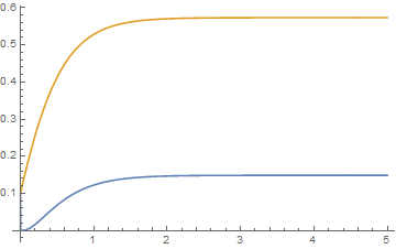
Here is the solution for initial conditions of $(x_0,y_0)=(0.1,0.1)$

q[x_, y_] := 1 - x (1 + Exp[1/y ]);
p[x_, y_] := 1 - y (1 + y Exp[x/ y]); 
sol = NDSolveValue[{x'[t] == q[x[t], y[t]], y'[t] == p[x[t], y[t]], 
    x[0] == 0.1, y[0] == 0.1}, {x[t], y[t]}, {t, 0, 5}];
Plot[{sol[[1]], sol[[2]]}, {t, 0, 5}]

I now add gaussian white noise to the first equation, and wish to solve $$dx = \left(1-x(t)\left(1+e^{-y(t)}\right)\right)dt+\sigma dW(t)$$ $$dy=\left(1-y(t)\left(1+e^{\frac{x(t)}{y(t)}}\right)\right)dt$$ $$dW(t) = \eta(t)\sqrt{dt}$$

where $\eta(t)$ is an uncorrelated white noise.

\[Sigma] = 0.1;
sol2 = RandomFunction[ItoProcess[{
     \[DifferentialD]x[t] == 
      1 - x[t] (1 + Exp[1/y [t]]) + \[Sigma]  \[DifferentialD]w[t],
     \[DifferentialD]y[t] == 1 - y[t] (1 - y[t] Exp[x[t]/ y[t]])}, {x[
      t], y[t]}, {{x, y}, {0.1, 0.1}}, t, 
    w \[Distributed] WienerProcess[]], {0, 5, 0.01}];

ListLinePlot[sol2]

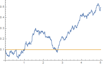
but I get results that seems independent of the deterministic solution itself

I would expect noise fluctuating around the deterministic solution of both state variables. In fact when I take \[Sigma]=0 I get a flat line of the initial condition, while I expect the deterministic solution itself.

Obviously I'm doing something wrong here. Since this is an over simplification of a larger problem I'm working on, I will appreciate if you could point along your answer what is the best way in your opinion to treat SDE's in mathematica.

Answer 1

A few things:

1) The second equation doesn't match the ODEs as noted by @b.gatessucks.

2) You need to use \[DifferentialD]t on the right hand sides.

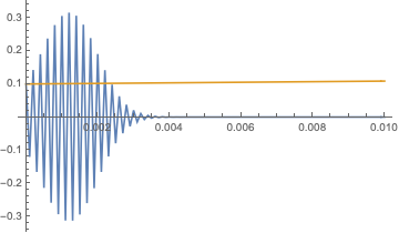
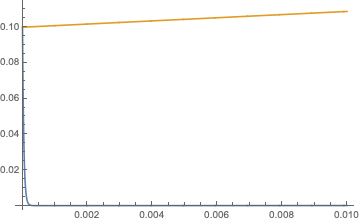
3) x[t] approaches zero very quickly in the solution to the ODEs. This makes me worried about the step size in RandomFunction[ItoProcess[]]. First, without noise:

sol2 = RandomFunction[ItoProcess[{
  \[DifferentialD]x[t] == (1 - x[t] (1 + Exp[1/y[t]])) \[DifferentialD]t,
  \[DifferentialD]y[t] == (1 - y[t] (1 + y[t] Exp[x[t]/y[t]])) \[DifferentialD]t},
  {x[t], y[t]}, {{x, y}, {0.1, 0.1}}, t,
  w \[Distributed] WienerProcess[0, σ]], {0, 0.01, dt}];

dt=0.001 fails. dt=0.0001 starts out badly, but manages to get it under control:

ListLinePlot[sol2, PlotRange -> All]

dt=0.00001 finally looks smooth like the NDSolve solution:

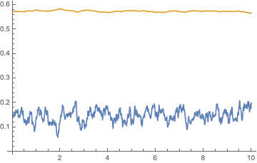
I think adding noise when x[t] is close to zero is probably too risky, so here's a solution that starts near the deterministic equilibrium. Note that we don't need the small steps in this neighborhood.

σ=0.1;
sol2 = RandomFunction[ItoProcess[{
  \[DifferentialD]x[t] == (1 - x[t] (1 + Exp[1/y[t]])) \[DifferentialD]t
    + \[DifferentialD]w[t],
  \[DifferentialD]y[t] == (1 - y[t] (1 + y[t] Exp[x[t]/y[t]])) \[DifferentialD]t},
  {x[t], y[t]}, {{x, y}, {0.149, 0.574}}, t,
  w \[Distributed] WienerProcess[0, σ]], {0, 10, 0.01}];
ListLinePlot[sol2, PlotRange -> All]