Solving a system of delayed partial differential equations

Question

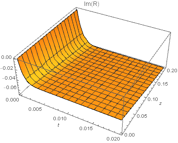
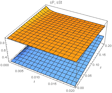
Dear (more advanced) users of Mathematica,

I'm still a beginner and currently trying to solve a system of delayed partial differential equations. Two of them describe the evolution of of two optical fields ($s_\text{P}$ and $s_\text{St}$) along a waveguide (position z):

(1) $\frac{\partial s_\text{P}\left(z,t\right)}{\partial z}=i \kappa_\text{S} R\left(z,t\right) s_\text{St}(z,t)$, and (2) $\frac{\partial s_\text{St}\left(z,t\right)}{\partial z}=i \kappa_\text{S} R^*\left(z,t\right) s_\text{P}\left(z,t\right)$.

These equation are coupled by the amplitude $R\left(z,t\right)$ of vibrations driven by the optical fields, which itself depends on time:

(3) $\frac{\partial R\left(z,t\right)}{\partial t} + \frac{\Gamma}{2} R\left(z,t\right) = i \kappa_\text{R} s_\text{P}\left(z,t\right) s_\text{St}^* \left(z,t\right)$.

I can obtain the steady-state solution ($\partial R/\partial t =0$) very easily by putting (3) into (1),(2) and applying NDSolve and the boundary conditions ($s_0\left(0,t\right) = \sqrt{0.9}$ and $s_\text{-1}(0,t)=\sqrt{0.1}$) to these two equations. But what I'd be interested in is the build-up of R over time. If I simply integrate (3) with $R(z,0) = 0$, I end up with an "delayed PDE" error.

Does anyone have an idea how I could proceed?

Thanks for your help in advance!

EDIT: This is my kind of naive code to solve this problem:

    (*DEFINE ALL THE CONSTANTS*)

Clear[ΩR, αS, κR, κS, γR, sar, c0];
ω0 = 2*Pi*2.99792458*10^8/(1.55*10^(-6));   (*optical frequency in Hz*)
c0 = 2.99792458*10^8;                       (*speed of light in vacuum*)
ΩR = 2*Pi*5.611*10^6;                       (*mechanical frequency in Hz*)
γR = 2*Pi*400;                              (*damping rate/linewidth in Hz*)
κS = -219.666*0.1;                          (*coupling rate*)
κR = κS*((c0*ΩR)/ω0)                        (*coupling rate*)  

(*SET UP PDEs TO SOLVE*)

Clear[sP, sSt, eqs, vars, bcs];
eqs = {{D[sP[z, t], z] == I κS*(I κR Exp[-γR*t/2]*
    Integrate[sP[z, d]*Conjugate[sSt[z, d]]*Exp[γR*d/2], {d, 0, t}])*sSt[z, t]},
       {D[sSt[z, t], z] == I κS*Conjugate[I κR Exp[-γR*t/2]*
    Integrate[sP[z, d]*Conjugate[sSt[z, d]]*Exp[γR*d/2], {d, 0, t}]]*sP[z, t]}}
vars = {sP[z, t], sSt[z, t]};      (*variables to solve for*)
bcs = {sP[0, t] == Sqrt[0.9], sSt[0, t] == Sqrt[0.1]};   (*boundary conditions at z=0*);
NDSolve[{eqs, bcs}, vars, {t, 0, 0.02}, {z, 0, 0.2}]

EDIT 2: Defining the integration of R as a function outside the NDsolve-block also seems to work.

(*DEFINE ALL THE CONSTANTS*)

Clear[ΩR, αS, κR, κS, γR, sar, c0];
ω0 = 2*Pi*2.99792458*10^8/(1.55*10^(-6));   (*optical frequency in Hz*)
c0 = 2.99792458*10^8;                       (*speed of light in vacuum*)
ΩR = 2*Pi*5.611*10^6;                       (*mechanical frequency in Hz*)
γR = 2*Pi*400;                              (*damping rate/linewidth in Hz*)
κS = -219.666*0.1;                          (*coupling rate*)
κR = κS*((c0*ΩR)/ω0)                        (*coupling rate*)  


R[t_, P_, S_] := I κR Exp[-γR*t/2]* Integrate[P*Conjugate[S]*Exp[γR*d/2], {d, 0, t}]

(*SET UP PDEs TO SOLVE*)

Clear[sP, sSt, eqs, vars, bcs];
eqs = {{D[sP[z, t], z] == 
    I κS*(R[t, sP[z, t], sSt[z, t]])*sSt[z, t]}, {D[sSt[z, t], 
     z] == I κS*Conjugate[R[t, sP[z, t], sSt[z, t]]]*sP[z, t]}}
vars = {sP[z, t],sSt[z, t]};(*variables to solve for*)
bcs = {sP[0, t] == Sqrt[0.9], sSt[0, t] == Sqrt[0.1]};(*boundary conditions for input fields at z=0*);
sol = NDSolve[{eqs, bcs}, vars, {t, 0, 0.003}, {z, 0, 0.1}]

(* GENERATE PLOTS *)

DensityPlot[sP[z, t]^2 /. sol, {t, 0, 0.003}, {z, 0, 0.1}, 
 ColorFunction -> "Rainbow", 
 FrameLabel -> {"Time (s)", "Propagation distance (m)"}, 
 PlotRange -> All, PlotLegends -> Automatic, PlotPoints -> 80]

DensityPlot[sSt[z, t]^2 /. sol, {t, 0, 0.003}, {z, 0, 0.1}, 
 ColorFunction -> "Rainbow", 
 FrameLabel -> {"Time (s)", "Propagation distance (m)"}, 
 PlotRange -> All, PlotLegends -> Automatic, PlotPoints -> 80]

DensityPlot[
 Abs[R[t, sP[z, t], sSt[z, t]]] /. sol, {t, 0, 0.003}, {z, 0, 0.1}, 
 ColorFunction -> "Rainbow", 
 FrameLabel -> {"Time (s)", "Propagation distance (m)"}, 
 PlotRange -> All, PlotLegends -> Automatic, PlotPoints -> 40]

Answer 1

Although NDSolve cannot solve this system of equations directly, it can produce the desired answer with some help. Here, we take advantage of the small size of the coupling to solve the system iteratively. First, initialize the problem.

ω0 = 2*Pi*2.99792458*10^8/(1.55*10^(-6));   (*optical frequency in Hz*)
c0 = 2.99792458*10^8;                   (*speed of light in vacuum*)
ΩR = 2*Pi*5.611*10^6;     (*mechanical frequency in Hz*)
γR = 2*Pi*400;                   (*damping rate/linewidth in Hz*)
κS = -219.666*0.1;               (*coupling rate*)
κR = κS*((c0*ΩR)/ω0);     (*coupling rate*)

eqsz = {{D[sP[z, t], z] == 0}, {D[sSt[z, t], z] == 0}};
vars = {sP[z, t], sSt[z, t]};   
bcs = {sP[0, t] == Sqrt[0.9], sSt[0, t] == Sqrt[0.1]};     
sz = vars /. Flatten@NDSolve[{eqsz, bcs}, vars, {t, 0, 0.02}, {z, 0, 0.2}];

Then solve the differential equations alternately for r[z, t] and for {sP[z, t], sSt[z, t]}. Six iterations is more than adequate for good convergence.

Do[
eqst = D[r[z, t], t] + r[z, t] γR/2 == I κR First[sz] Conjugate[Last[sz]];
sr = r[z, t] /. Flatten@NDSolve[{eqst, r[z, 0] == 0}, r[z, t], {t, 0, 0.02}, {z, 0, 0.2}];

eqsz = {{D[sP[z, t], z] == I κS*sr*sSt[z, t]},     
        {D[sSt[z, t], z] == I κS*Conjugate[sr]*sP[z, t]}};
bcs = {sP[0, t] == Sqrt[0.9], sSt[0, t] == Sqrt[0.1]};     
sz = vars /. Flatten@NDSolve[{eqsz, bcs}, vars, {t, 0, 0.02}, {z, 0, 0.2}];,
{i, 6}]

Plot3D[Im@sr, {t, 0, 0.02}, {z, 0, 0.2}, PlotLabel -> R, 
    AxesLabel -> {t, z}, PlotRange -> All]
Plot3D[sz, {t, 0, 0.02}, {z, 0, 0.2}, PlotLabel -> "sP, sSt", 
    AxesLabel -> {t, z}]

The computation takes a few seconds.