A few things:
The second equation doesn't match the ODEs as noted by @b.gatessucks.
You need to use
\[DifferentialD]ton the right hand sides.x[t]approaches zero very quickly in the solution to the ODEs. This makemakes me worried about the step size inRandomFunction[ItoProcess[]]. First, without noise:sol2 = RandomFunction[ItoProcess[{ [DifferentialD]x[t] == (1 - x[t] (1 + Exp[1/y[t]])) [DifferentialD]t, [DifferentialD]y[t] == (1 - y[t] (1 + y[t] Exp[x[t]/y[t]])) [DifferentialD]t}, {x[t], y[t]}, {{x, y}, {0.1, 0.1}}, t, w [Distributed] WienerProcess[0, σ]], {0, 0.01, dt}];
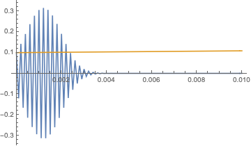
dt=0.001 fails. dt=0.0001 starts out badly, but manages to get it under control:
ListLinePlot[sol2, PlotRange -> All]

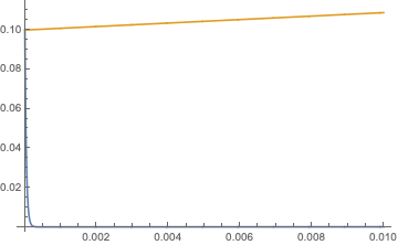
dt=0.00001 finally looks smooth like the NDSolve solution:

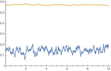
I think adding noise when x[t] is close to zero is probably too risky, so here's a solution that starts near the deterministic equilibrium. Note that we don't need the small steps in this neighborhood.
σ=0.1;
sol2 = RandomFunction[ItoProcess[{
  \[DifferentialD]x[t] == (1 - x[t] (1 + Exp[1/y[t]])) \[DifferentialD]t
    + \[DifferentialD]w[t],
  \[DifferentialD]y[t] == (1 - y[t] (1 + y[t] Exp[x[t]/y[t]])) \[DifferentialD]t},
  {x[t], y[t]}, {{x, y}, {0.149, 0.574}}, t,
  w \[Distributed] WienerProcess[0, σ]], {0, 10, 0.01}];
ListLinePlot[sol2, PlotRange -> All]

