Solution of a BVP by shooting method

Question

I have the next system of ODEs: $$ \frac{1}{2}\sigma^2 p''_n(x)+x p'_n(x)+p_n(x)-\frac{p_n(x)-p_{n-1}(x)}{\Delta t}=0,$$ $$p_1(a)=p(b)=0;\quad p_0(x)=0.1,\quad n=1.\dots N, $$ which was derived from the elliptic pde by method of lines: $$\frac{\partial p}{\partial t}=p+x\frac{\partial p}{\partial x}+\frac{1}{2}\sigma^2\frac{\partial^2 p}{\partial x^2},$$ $$lim_{x\rightarrow\pm \infty} p(x,t)=0,\quad \forall t.$$ Now I should set the border values: $a$ and $b.$ I want them to be as far from zero as possible. But the problem arises when I try to solve the system by method of shooting, that doesn't permit me to set them different from $a=0$, $b=1$.

n = 5;
h = 1/n;
U[x_] = Table[Subscript[u, i][x], {i, 0, n}] /. 
   Subscript[u, 0][x] -> g[x];
Eq = Table[Subscript[eq, i], {i, 0, n}];
\[Sigma] = 0.1;
a[x_, t_] = 1/2 \[Sigma]^2;
b[x_, t_] = x;
c[x_, t_] = -1;
d[x_, t_] = 1;
f[x_, t_] = 0;
g[x_] = 0.1;
\[Alpha][t_] = 0;
\[Beta][t_] = 0;
xl = -0.5;
xr = 0.5;
A=0;
B=1;
eqs = Table[Eq[[i]] =  1/(xr - xl)^2 a[x, h i ] D[U[x][[i]], {x, 2}] + 1/(xr - xl) b[x, h i ] D[U[x][[i]], x] - c[x, h i ] U[x][[i]] - d[x, h i ]  ((U[x][[i]] - U[x][[i - 1]])/h) - f[x, h i ] == 0, {i, 2, n + 1}];
bcs = Table[{U[A][[i]] == 0, U[B][[i]] == 0}, {i, 2, n + 1}]
sols = First[ NDSolve[{eqs, bcs}, U[x], x, Method -> {"Shooting", 
     "StartingInitialConditions" -> Table[(D[U[x][[i]], x] /. x -> 0) == 1, {i, 2, n + 1}]}]]

When I set $A=-1$ and change initial conditions for method of shooting I get the error:

NDSolve::bvluc: The equations derived from the boundary conditions are numerically ill-conditioned. The boundary conditions may not be sufficient to uniquely define a solution. If a solution is computed, it may match the boundary conditions poorly.

NDSolve::berr: The scaled boundary value residual error of 5.277001462096112`*^45 indicates that the boundary values are not satisfied to specified tolerances. Returning the best solution found.

I've also tried to rescale the system by inputing scale variables $xl$ and $xr$. But the same problem holds true. Only current values can be applied. Have no clue what's the problem can be - the analytical solution for the given pde exists uniquely.

Answer 1

The main issue with your code is very simple, you are trying to take your domain in $A\leq x\leq B$ and split it into $n$ equal sized pieces. These should have size $h=(B-A)/n$, but you are setting them to be size $h=1/n$. All you need to do for your code to not give errors is to define A and B first, and then set h=(B-A)/n.

It does seem very slow though for larger values of n, and you might want to use higher order derivative formulae.

Adapting some code I have for method of lines, but discretizing in $x$ instead of $t$ (have to take a lot of points here with the default settings, else error creeps in and the solutions blow up.):

A=-5;B=5;σ=0.1;
n=300;h = (B-A)/n; 
gridpts=(Range[A,B,h]);
P[t_] = Table[Subscript[p,i][t],{i,0,n}];
nDeriv[m_?NumericQ,fn_]:=NDSolve`FiniteDifferenceDerivative[m,gridpts, fn,DifferenceOrder->2];
psubs={p[x,t]:>nDeriv[0, P[t]],Derivative[Pattern[i,Blank[]],0][p][x,t]:>nDeriv[i,P[t]],Derivative[0,Pattern[i,Blank[]]][p][x,t]:>D[P[t],{t,i}],XX[x]:>gridpts};
eqn=D[p[x,t],t]==p[x,t]+ XX[x] D[p[x,t],x]+1/2 σ^2 D[p[x,t],x,x];
MoLeqns=Flatten@{First[nDeriv[0,P[t]]]==0,Most@Rest@Thread[(eqn/.psubs)],Last[nDeriv[0,P[t]]]==0};

(* find an initial perturbation from zero satisfies the boundary conditions *)

initsol=(a0+a1 x+a2 x^2)/.Solve[{p[A]==0,p[B]==0}/.p->Function[{x},(a0+a1 x +a2 x^2)]][[1]];


inits=Thread[P[0]==Table[initsol/.a0->-0.01,{x,gridpts}]];
lines=NDSolve[{MoLeqns,inits},Table[Subscript[p,i],{i,0,n}],{t,0,50}][[1]];
tend=lines[[1,2,1,1,2]];

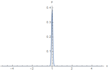
This gives a steady solution that has a spike at $x=0$ and rapidly decays outside that:

ListLinePlot[P[tend] /. lines, PlotRange -> All,  DataRange -> {A, B}, AxesLabel -> {"x", "p"}]

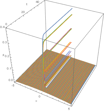
Or you can see how the individual lines behave:

ParametricPlot3D[Evaluate[Table[{A+ i h,t, Subscript[p,i][t] /.lines},{i,0,n}]],{t,0,tend}, PlotRange->All, AxesLabel->{"x","t","p"}]