Consider a function
f[x_, Z_, α_, mN_, q_, R_, S_] =
  Assuming[mN > 0 && x > 0,
   9*α*Z^2/(2*Pi)*((1 + (1 - x)^2)/x)*
    (q^2 - x^2 mN^2)/q^4*
    SphericalBesselJ[1,
      R*q]^2/(R*q)^2*
    Exp[-q^2*S^2]];
It is defined in the domain $$ \text{max}[2\cdot 10^{-5}, x\cdot m_{N}]< q< q_{\text{max}} = 4.49/5, \quad 10^{-9}<x <q_{\text{max}}/m_{N} $$ I'm trying to obtain the interpolation of numerical integral $$ \int \limits_{q_{\text{min}}}^{q_{\text{max}}}dq^{2}f[x,42,1/137,100,q,5,0.726] $$ for the given value of x. Namely, I write
g1 =
  Table[{x,
    NIntegrate[
     f[x, q, 42, 1/137, 100, 5, 0.726]*2*q, {q,
      Max[100*x, 2*10^-5], 4.49/5}]}, {x, 10^-9, 4.49/(5*100), 10^-4}];
g[x_] = Interpolation[g1 ][x]
Finally, I want to draw a plot of the function g[x]. I write
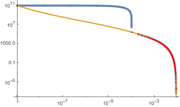
LogLogPlot[g[x], {x, 10^-9, 4.49/(5*100)}, PlotRange -> All]
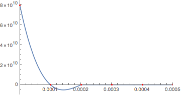
And I see discontinuous plot. The point of discontinuity strongly depends on the table step size (I've tried from $10^{-7}$ to $10^{-2}$). From the other side, if I simply write
LogLogPlot[
 NIntegrate[
  Re[f[x, q, 42, 1/137, 100, 5, 0.726]]*2*q, {q,
   Max[100*x, 2*10^-5], 4.49/5}], {x, 10^-9, 4.49/(5*100)},
 PlotRange -> All],
then the plot is smooth.
How to obtain correct interpolation?
The code sample is
 f[x_, Z_, α_, mN_, q_, R_, S_] =
      Assuming[mN > 0 && x > 0,
       9*α*Z^2/(2*Pi)*((1 + (1 - x)^2)/x)*
        (q^2 - x^2 mN^2)/q^4*
        SphericalBesselJ[1,
          R*q]^2/(R*q)^2*
        Exp[-q^2*S^2]];

    g1 =
      Table[{x,
        NIntegrate[
         f[x, 42, 1/137, 100,q, 5, 0.726]*2*q, {q,
          Max[100*x, 2*10^-5], 4.49/5}]}, {x, 10^-9, 4.49/(5*100), 10^-4}];
    g[x_] = Interpolation[g1 ][x]

    LogLogPlot[g[x], {x, 10^-9, 4.49/(5*100)}, PlotRange -> All]


PhotonDFx? Please provide sample code that can be evaluated from start to finish. $\endgroup$fevaluates to zero: i.sstatic.net/qYsle.png -- Ing1, you've substituted the argumentqinto the slot forZ. Perhaps that's a mistake? (If not, I get a constant0.for the value ofg, not a discontinuous function.) $\endgroup$Plot[g[x], {x, 10^-9, 4.49/(5*100)}, PlotRange -> All]and you'll see that the interpolation goes negative. That's why the log-log plot has a gap. TryInterpolationOrder -> 2orInterpolationOrder -> 1. $\endgroup$