Map volumetric data onto an isosurface

Question

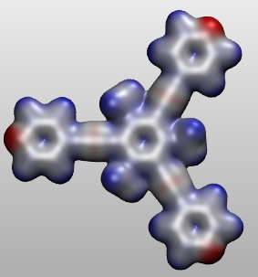
this question originates from an attempt to visualize molecular electrostatic potentials, but hopefully should be of general interest.

Suppose that you have two sets of data, S1 and S2. Each set consists of a certain number of 3D points (x,y and z coordinates) each one characterised by a certain (scalar) value. The 3D points are the same for the two datasets - the only difference is the scalar values associated with said points.

What I would like to do is to build a 3D isosurface from one of these two datasets (S1, by selecting a specific isovalue) and then map the second dataset (S2) onto this particular isosurface. In other words, to "color" the isosurface according to the S2.

Within a more "chemical" point of view, I would like to map the electrostatic potential (S2) onto a specific isosurface of the electronic density (S1). This can be done by a number of visualization tools (here you'll find more or less what should be obtained in this particular case), but I would really like to take advantage of Mathematica to play around with 3D countours and the like.

In principle, there exist a Wolfram Demonstration Project about this. However, there is very little Mathematica used in that example, all the tricky bits are taken care of by external software - including the mapping of the electrostatic potential onto the isosurface of the electronic density.

In practice, the starting point consists into two .cube files, which can be read into Mathematica and plot via a CubePlot function (stolen from here) which in turn takes advantage of ListContourPlot3D.

I attach the two relevant .cube files (S1 and S2) and a (rather embarassing...) notebook which goes as far as reading S1 and S2 from the two .cube files and plotting the S1 isosurface of interest. In principle it should be possible (he said confidently...) to select a specific isovalue of S1 via a specific value of Contours (this I have done) while coloring the surface via the S2 data... but that's where I'm presently stuck.

Any help would be much appreciated indeed - happy to discuss any of this in greater detail!

---

Alas,

I am afraid this is not the end of the story.

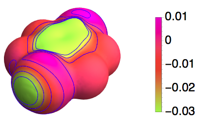
Playing around a bit I realised that the distribution of the electrostatic potential (the color map) for the molecule in the example above was not symmetric as it should have been. Easy to miss that for a very small molecule, but for larger ones the issue becomes immediately clear.

This is the correct result (obtained by using VMD) for a slightly larger molecule:

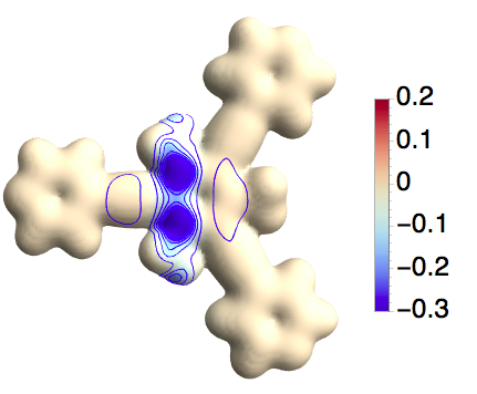
While this is what I get using Mathematica (here you can find the notebook and the relavant files):

Obviously there is something very wrong going on in here. I have played around with a number of things. I believe the problem lies somewhere in the ColorFunction bit:

ColorFunction -> Function[{x, y, z}, ColorData["ThermometerColors", Rescale[esp[x, y, z], espRange]]]

which in turn relies on the interpolation of the electrostatic potential:

dataRangeESP = Map[MinMax, {espxg, espyg, espzg}]; esp = ListInterpolation[Transpose[espdata, {3, 2, 1}], dataRangeESP];

The isosurfaces for the electron density (and for the electrostatic potential itself, I have tried...) are represented correctly - it is "just" the coloring of said isosurfaces with the electrostatic potential that for some reason gives the wrong result.

Any help would be very much appreciated indeed!

Answer 1

The solution takes advantage of Jason B.'s suggestions - hats off to him!

The full notebook is available here.

In summary, the two .cube files (containing the electron density and the electrostatic potential - on the same 3D grid) are read via a ReadCube function (stolen from here).

A particular isosurface of the electron density is then chosen via the Contours option of ListContourPlot3D. The electrostatic potential is mapped onto said surface via the ColorFunction directive of ListContourPlot3D.

Here follows the relevant snippet:

dataRange = Map[MinMax, {xg, yg, zg}]; (* the 3D range *)
espRange = {-0.03, 0.01}; (* the range of values for the electrostatic potential*)
esp = ListInterpolation[Transpose[espdata, {3, 2, 1}], dataRange]; (* Interpolate the electrostatic potential so that we can use it to color the electron density isosurface via the ColorFunction directive *)
vp = ViewPoint -> {1.3, -2.4, 2.0};
labels = Directive[FontSize -> 24, Black, FontFamily -> "Helvetica"];
densityPlot = 
Legended[ListContourPlot3D[Transpose[cubedata, {3, 2, 1}], 
   DataRange -> dataRange, Contours -> {0.001}, PlotRange -> Automatic,
   BoxRatios -> Automatic, Axes -> False, vp, Boxed -> False, 
   MeshStyle -> Directive[Thickness[0.0075], Blue]
   , ColorFunction -> 
    Function[{x, y, z}, 
     ColorData["NeonColors", Rescale[esp[x, y, z], espRange]]], 
   ColorFunctionScaling -> False, MeshFunctions -> {esp[#, #2, #3] &},
Mesh -> {{-0.03, -0.02, -0.01, 0.00, 0.01}}], 
BarLegend[{"NeonColors", espRange}, LabelStyle -> labels]]

And here is the final result:

To my (admittedly quite limited...) knowledge, this is an incredibly quick way to generate this sort of electrostatic potential maps - which look so much better if compared to the vast majority of what you get out of dedicated visualization software.