SphericalPlot3D of an OblateSpheroid via coordinate transformation

Question

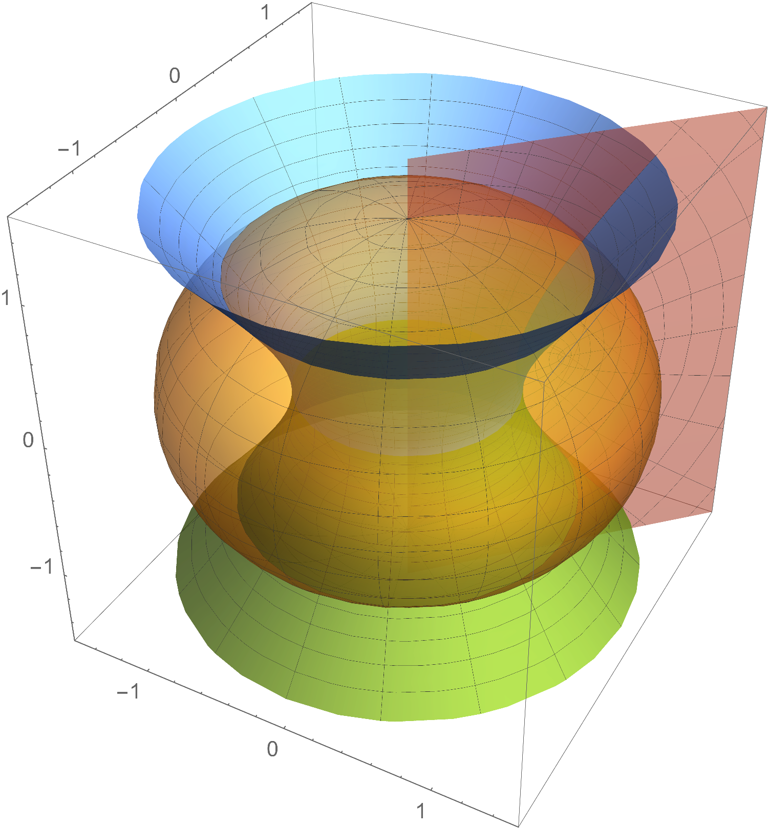
This is an effort to reproduce an ellipse and a hyperbola of revolution from OblateSpheroidal coordinates with constant $\eta$ and $\theta$ .

My approach consisted in getting a Coordinate Transformation of OblateSpherodcal Coordinate[] function converts to Spherical coordinate then do a SphericalPlot3D.

mapping = 
 CoordinateTransformData[{{"OblateSpheroidal", 1}, 3} -> "Spherical",
   "Mapping"]
sph = mapping@
  CoordinateChartData[{{"OblateSpheroidal", {\[FormalA]}}, 
    "Euclidean", 3}, "StandardCoordinateNames"]
SphericalPlot3D[{{sph[[1]]}, {sph[[3]]}}, {\[Xi], 0, Pi}, {\[Eta], 0, 
  3 Pi/2}]

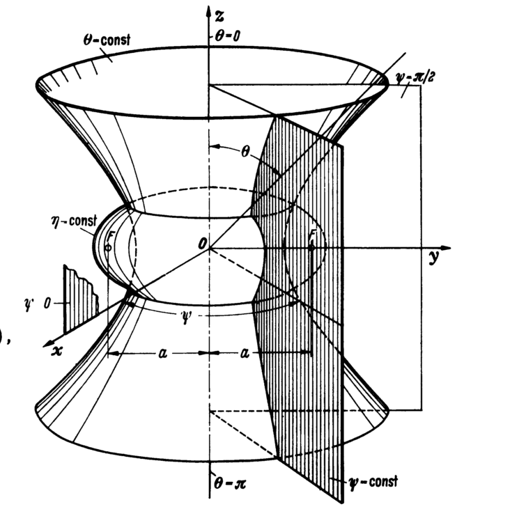
By the plot returns empty. Here is a nice drawing of what I am expectating from the plot.

UPDATE 1

Thanks to the contribution from participating members, was able to clear some fundamental issues related to distinguish between string and symbols. Here is a cleaner version of the code:

fromOblatetoSpherical = 
  CoordinateTransformData[{{"OblateSpheroidal", 1}, 3} -> "Spherical",
    "Mapping"];
CoordinateChartData[{{"OblateSpheroidal", {\[FormalA]}}, "Euclidean", 
   3}, "StandardCoordinateNames"];
sph = fromOblatetoSpherical@%
sph2 = Simplify[sph /. x_String :> ToExpression[x]]
SphericalPlot3D[{sph2[[1]], sph2[[3]]}, {\[Xi], 0, Pi}, {\[Eta], 0, 
  3 Pi/2}, PlotStyle -> 
  Directive[Orange, Opacity[0.5], Specularity[White, 10]], 
 PlotRange -> All, Mesh -> None, PlotPoints -> 50]

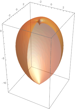
The result is not quite what I am expecting , since I want to construct a Ellipsoid and the rotated Hyperbola as the figure 2. Therefore, I need the 2 surfaces in the plot .

UPDATE 2

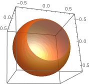
Enhanced code.. I can not figure out why get spheres and not ellipsoid.

fromOblatetoSpherical = 
  CoordinateTransformData[{{"OblateSpheroidal", 1}, 3} -> "Spherical",
    "Mapping"];
CoordinateChartData[{{"OblateSpheroidal", {\[FormalA]}}, "Euclidean", 
  3}, "StandardCoordinateNames"]
sph = fromOblatetoSpherical@%
sph2 = Simplify[sph /. x_String :> ToExpression[x]]
SphericalPlot3D[
   sph2[[1]] = #/5, {\[Eta], 0, 3 Pi/4}, {\[CurlyPhi], 0, 2 Pi}, 
   PlotStyle -> 
    Directive[Orange, Opacity[0.7], Specularity[White, 10]], 
   PlotRange -> All, ImageSize -> Small, Mesh -> None, 
   PlotPoints -> 50] & /@ {-1, 3, 6, 8, 12}

Here is one of the plot3D images

Answer 1

I'm afraid your approach is flawed. SphericalPlot3D[r,t,p] plots r[t,p], where t and p are assuming to be independent spherical angles. But you don't want t and p to be independent, you want them to be functions of oblate spheroidal coordinates. (Incidentally, this is also why you're getting spheres in your last version: you're telling it to plot r==constant independent of theta and phi, which is clearly a sphere.)

It's much easier to create the mapping to Cartesian coordinates, then use ParametricPlot3D holding one of your independent variables constant. For example:

trans = CoordinateTransformData[{{"OblateSpheroidal", 1}, 3} -> "Cartesian", "Mapping"];
ParametricPlot3D[{trans[{1, η, φ}]}, {η, 0, Pi}
  , {φ, -π, π}, PlotStyle -> Opacity[.5]
];
ParametricPlot3D[{None, trans[{ξ, Pi/4, φ}], trans[{ξ, 3 Pi/4, φ}]}
  , {ξ, 0, 1.4}, {φ, -π, π}, PlotStyle -> Opacity[.8]
];
ParametricPlot3D[{None, None, None, trans[{ξ, η, Pi/4}]}
  , {ξ, 0, 2}, {η, 0, π}, PlotStyle -> Opacity[.5]
];
Show[{%, %%, %%%}, PlotRange -> 1.5]

In each plot, I hold one of the variables fixed, and let the others range the entire or a reasonable interval. Also, notice how I'm using None to get the correct sequence of colors when I assemble it all together. The result looks like this: