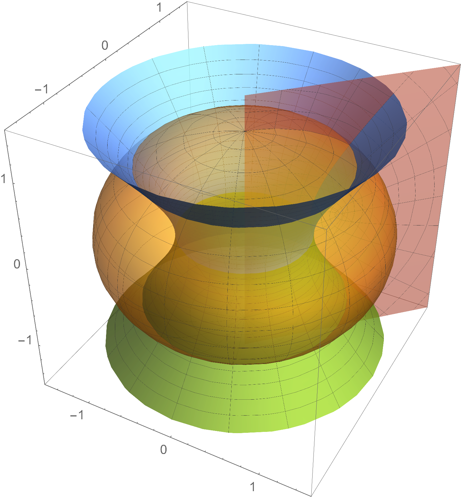
I'm afraid your approach is flawed. SphericalPlot3D[r,t,p]SphericalPlot3D[r,t,p] plots r[t,p]r[t,p], where tt and pp are assuming to be independent spherical angles. But you don't want tt and pp to be independent, you want them to be functions of oblate spheroidal coordinates. (Incidentally, this is also why you're getting spheres in your last version: you're telling it to plot r==constantr==constant independent of theta and phiphi, which is clearly a sphere.)
It's much easier to create the mapping to Cartesian coordinates, then use ParametricPlot3DParametricPlot3D holding one of your independent variables constant. For example:
trans = CoordinateTransformData[{{"OblateSpheroidal", 1}, 3} ->
    "Cartesian", "Mapping"];
ParametricPlot3D[{trans[{1, \[Eta]η, \[CurlyPhi]φ}]}, {\[Eta]η, 0, Pi}
   Pi}, {\[CurlyPhi]φ, -\[Pi]π, \[Pi]π}, PlotStyle -> Opacity[.5]];5]
];
ParametricPlot3D[{None, trans[{\[Xi]ξ, Pi/4, \[CurlyPhi]φ}],
   trans[{\[Xi]ξ, 3 Pi/4, \[CurlyPhi]φ}]}
  , {\[Xi]ξ, 0,
   1.4}, {\[CurlyPhi]φ, -\[Pi]π, \[Pi]π}, PlotStyle -> Opacity[.8]];8]
];
ParametricPlot3D[{None, None, None,
   trans[{\[Xi]ξ, \[Eta]η, Pi/4}]}
  , {\[Xi]ξ, 0, 2}, {\[Eta]η, 0, \[Pi]π},
  PlotStyle -> Opacity[.5]];5]
];
Show[{%, %%, %%%}, PlotRange -> 1.5]
In each plot, I hold one of the variables fixed, and let the others range the entire or a reasonable interval. Also, notice how I'm using None to get the correct sequence of colors when I assemble it all together. The result looks like this:

