You are looking for ideas, so I will venture a partial solution in the hope it might inspire something useful. The idea presented here is to exploit a statistical model of the heartbeat intervals as a way to test the goodness of any attempted clustering of the data.
The approach is general, because it is based on maximum likelihood methods, but I will illustrate it for a particularly simple, tractable, and (possibly) applicable case. (I hold out no hope that the following model is particularly correct; I only maintain it may be a good enough approximation to afford some insight and perhaps improve solutions to the problem.)
Let us suppose that the heartbeat intervals are independent and identically distributed according to some member $f_\theta$ of a parametric family, such as a Normal distribution (where $\theta=(\mu, \sigma)$ gives the mean and standard deviation). Let us also suppose that, independent of that process, there is another parameterized discrete random variable with values in the nonnegative integers giving the number of places where which each interval is broken. Let its probability function be $p_\lambda$: presumably, its expectation is close to $0$. Finally, let us suppose that conditional on these two processes, a third distribution governs the proportions in which the intervals are broken. Let its probability function be $u_\phi$.
When $f$ is Normal, $p$ is Poisson, and $u$ is uniform, the problem becomes analytically tractable. (Such tractability is not necessary, but it speeds the execution of the program and can provide insight into what's going on.) To write the log likelihood--which we intend to maximize--suppose that the data have already been grouped into sequences corresponding to a single beat. The contribution to the log likelihood from such a group $(x_i)$, $i=1,2,\ldots,k$, is
$$\Lambda = \Bigl[-\frac{(\sum x_i - \mu)^2}{2 \sigma^2} - \frac{1}{2} \log(2 \pi \sigma^2)\Bigr] + [-\lambda + k \log(\lambda) - \log(k!)] + [\log(k!)].$$
From left to right, the terms are grouped according to the contributions from the Normal distribution, the Poisson, and the uniform. Contingent on this grouping, closed formulas for values of $\mu, \sigma$, and $\lambda$ which maximize the log likelihood can be derived (and are simple): $\hat{\mu}$ is the mean of the group sums, $\hat{\lambda}$ is $1$ greater than the ratio of number of observations to number of groups, and $\hat{\sigma}$ is the standard deviation of the group sums about $\hat{\mu}$.
To enable automatic identification of heartbeats, it may be best to represent the groups of data by means of an indicator (0-1) vector $y$: the cumulative sums of $y$ designate the groups. Thus, $y$ is $1$ at the start of each group of readings and is $0$ for intermediate readings. Equivalently, $y$ is the indicator of the actual beats. Let $\Lambda^*(y)$ designate the maximized log likelihood for the grouping given by $y$.
What we need is a way to find such a $y$ for which $\Lambda^*(y)$ is as large as possible. This is a nonlinear binary optimization program. It seems a little tricky, but there's a natural underlying structure to the problem making it feasible. Generally, many heartbeats can be clearly identified using heuristics such as those suggested in other answers to the question. All we have to do is vary $y$ slightly around the endpoints of some of the more problematic groupings.
Let's see how this might play out in practice. Begin with the sequence of $215$ observations:
data = Flatten[Import["https://dl.dropbox.com/u/1989758/beattobeatdata.txt", "Table"]];
ListPlot[data, PlotRange -> {Full, Full}, AxesOrigin -> {0, 0},
    PlotStyle -> PointSize[0.0125], AxesLabel -> {"Index", "Interval"}]
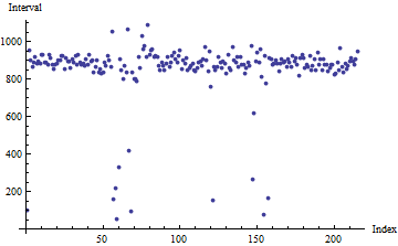
A break in its histogram suggests a starting threshold for identifying overly short intervals:
Histogram[data]
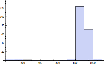
Somewhere around $550$ will do. We take this as an initial indicator and, preparatory to the next step, save it:
y = ConstantArray[1, Length[data]];
y[[ Flatten[Position[data, a_ /; a < 550]]]] = 0;
x = y;
Before going on, we need to be able to maximize $\Lambda(y)$. This function returns an array given the best value of the log likelihood and the associated parameter values, $\{\Lambda^*(y), \{\{\hat{\mu}, \hat{\sigma}^2\}, \hat{\lambda}\}$.
maxLogL[data_, x_] := Module[{logL, k = Total[x], n = Length[x], \[Lambda], \[Mu], \[Sigma]2},
   \[Lambda] = n/k - 1;
   \[Mu] = Total[data]/k;
   \[Sigma]2 = Total[(Total /@ (First /@ # & /@
      GatherBy[{data, Accumulate[x]}\[Transpose], Last]) - \[Mu])^2] / k;
   {f[data, {x, {\[Mu], \[Sigma]2}, \[Lambda]}], {{\[Mu], \[Sigma]2}, \[Lambda]}}
   ];
It calls f to compute $\Lambda^*(y)$:
f[data_, {x_, {\[Mu]_, \[Sigma]2_}, \[Lambda]_}] := Module[{logL},
   logL = Function[{z}, -(1/2.) (Total[z] - \[Mu])^2 / \[Sigma]2 - (1/2.) Log[2. \[Pi] \[Sigma]2]
     - \[Lambda] + (Length[z] - 1) Log[\[Lambda]]];
   Total[logL /@ (First /@ # & /@  GatherBy[{data, Accumulate[x]}\[Transpose], Last])]
   ];
The maximum log likelihood associated with the initial value of $y$ equals $-1293.79$:
maxLogL[data, y] // N
{-1293.79, {{898.461, 12047.1}, 0.0539216}}
Let's try to improve this by changing just one entry in $y$ at a time:
For[y = x; lMax = maxLogL[data, y] // First; i = 1, i <= Length[x], i++,
  y[[i]] = 1 - x[[i]];
  lMax0 = First[maxLogL[data, y]];
  {lMax, y[[i]]} = If[ lMax0 < lMax, {lMax, x[[i]]}, {lMax0, y[[i]]}]
  ];
lMax
-1172.63
That's a tremendous improvement in $\Lambda^*$ from $-1293.79$ to $-1172.63$. (Increases of $2$ or so are often considered "significant." Remember, these numbers are natural logarithms.) By inspection of the data (using plots and tables), we can do a little better still:
y[[147]] = 1; y[[148]] = 0; maxLogL[data, y] // N
{-1142.2, {{889.738, 2671.79}, 0.0436893}}
The large increase of $30.4$ in $\Lambda^*$ demonstrates this change in the clustering was worthwhile.
Let's take a look at the results by plotting the current estimate of the heartbeats represented by $y$:
ListPlot[Total /@ (First /@ # & /@
GatherBy[{data, Accumulate[y]}\[Transpose], Last]),
  PlotRange -> {Full, Full}, AxesOrigin -> {0, 0},
  PlotStyle -> PointSize[0.0125], AxesLabel -> {"Beat", "Interval"}]
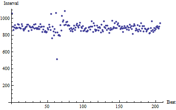
It is wise to explore the log likelihood function. The mean of $889.738$ looks solid, so let's draw contours of the log likelihood by varying the other two parameters, $\sigma$ and $\lambda$:
ContourPlot[f[data, {y, {889.738, \[Sigma]^2}, \[Lambda]}],
  {\[Lambda], 0.02, 0.08}, {\[Sigma], 46, 58}],
  Epilog -> {Red, PointSize[0.015], Point[{0.0436893, Sqrt[2671.79]}]}
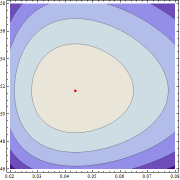
The contour interval is $1$. We can therefore expect that this plot shows, approximately, a $95$% contour ellipse for $(\lambda, \sigma)$. The conclusion is that:
The mean heartbeat interval is $889.7$. It is likely between $882$ and $898$ (as indicated by similar contour plots of $\mu$ versus $\sigma$ and $\mu$ versus $\lambda$, not shown here).
The standard deviation of the intervals is $51.7 = \sqrt{2671.79}$ and is likely between $46$ and $58$ or so.
The rate at which beats are interrupted is $\hat{\lambda} = 0.044$ and is likely between $0.02$ and $0.08$ or so.
There are some outlying data around indexes $50$ to $70$ in the raw data, as the previous list plot shows: this is a clear violation of the parametric assumptions of these calculations. Nevertheless, it appears they have done a good job of characterizing the data overall and of guiding us to a good solution of the original problem of clustering the data and classifying them into heartbeats and non-heartbeats.
There are obvious improvements to be made. The first is that this probability model is obviously deficient: any anomalies in the data are likely to be positively correlated; the variation of heartbeat intervals is not Normal; the mean interval might change over time. Introducing parameters to handle these complications is a matter of computational complexity but creates no new conceptual or computational problems.
The second is that I have not proposed an automated way to find $y$. As far as I can tell, Mathematica has no built-in procedure to handle this kind of optimization. It should succumb easily to a genetic algorithm, simulated annealing, or perhaps even a dynamic program, but I haven't the time to do that coding.
(My code is awfully quick and dirty too, but at this stage that is of little import.)
I have offered this account because the idea of using a likelihood maximizer to help evaluate possible solutions ought to be applicable no matter what solution method is ultimately adopted. By using a probability model it will be less ad hoc than most attempts and can even provide some insight into the heartbeat process itself.



Splitworks on your small example:Split[data, Abs[#2 - #1] < 300 &]. However, more data is required to test how robust a simple, single threshold toSplitis... $\endgroup$300to something else. I think it's difficult to implement it in a function that handles lots of different data. And i added a link to some actual data. $\endgroup$