How can one generate an open-ended sequence of low-discrepancy points in 3D?

Question

I'd like a low-discrepancy sequence of points over a 3D-hypercube $[-1,1]^3$, but don't want to have to commit to a fixed number $n$ of points beforehand, that is just see how the numerical integration estimates develop with increasing numbers of low-discrepancy points.

I'd like to avoid have to start all over again, if the results with a fixed $n$ are unsatisfactory. Of course, one could just employ random numbers, but then the convergence behavior would be poorer.

Since in his answer below, Martin Roberts advances a very interesting, appealing approach to the open-ended low-discrepancy problem, I’d like to indicate an (ongoing) implementation of his approach I’ve just reported in https://arxiv.org/abs/1809.09040 . In sec. XI (p. 19) and Figs. 5 and 6 there, I analyze two problems—one with sampling dimension $d=36$ and one with $d=64$—both using the parameter $\bf{\alpha}_0$ set to 0 and also to $\frac{1}{2}$. To convert the quasi-uniformly distributed points yielded by the Roberts’ algorithm to quasi-uniformly distributed normal variates, I use the code developed by Henrik Schumacher in his answer to Can I use Compile to speed up InverseCDF?

Three years after my posting of the original question, I've been pursuing a problem which involves the implementation of the precise 3D procedure Martin Roberts gave in his extensive answer below. However, in the interest of increased accuracy/precision, I chose (using WorkingPrecision->20) for the "generalized golden ratio" constant the value $\phi_3=1.2207440846057594754$, rather than the indicated 1.2207440846. So, for the recurrence sequence $R:\bf{t}_{n+1} =\bf{t}_n+ \bf{\alpha}\mod 1$, rather than \begin{equation} \alpha= (0.819173,0.671044,0.549700), \end{equation} I employ \begin{equation} \alpha =(0.81917251339616443970, 0.6710436067037892084, 0.5497004779019702669). \end{equation} I've now run 1,800,000,000 iterations of the procedure, recording results at intervals of 100 million. I'm estimating nine quantities, for three of which I already know the exact values, that is \begin{equation} \left\{\frac{8 \pi }{27 \sqrt{3}},\frac{1}{81} \left(27+\sqrt{3} \log \left(97+56 \sqrt{3}\right)\right),\frac{2}{81} \left(4 \sqrt{3} \pi -21\right)\right\}= \end{equation} \begin{equation} \{0.53742203384717565944, 0.44597718463717723667, \ 0.018903515328657140917\}. \end{equation} Now, after 1,700,000,000 iterations, the ratios of my estimates to the three known values were \begin{equation} \{0.99999434335413677936,1.0000002215189648742,0.99998070678044792723\}, \end{equation} while after 1,800,000,000 iterations the ratios were \begin{equation} \{0.99999956436935409259,1.0000009222826007255,0.99995924493777645856\} \end{equation} So, the first of the three estimates improves, while the other two "deteriorate".

So, what is the relation of my initial choice of WorkingPrecision->20 to the quality of the estimates? In particular, my concern is that since at every iteration, the command FractionalPart is performed, that conceivably at some iteration, rather than obtaining, say 0.9999999999999999, one might obtain 0.0000000000000001--leading to subsequent "severe" (?) deterioration. If I had chosen WorkingPrecision->48 say instead, might the quality have possibly been different?--at least, have increased confidence. (Maybe I should redo the calculations--and see what happens.)

So, to what extent is the Martin Roberts procedure (and/or other quasirandom ones) subject to accuracy/precision issues? How "robust" is it?

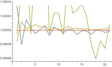
Here's a ListPlot of the accuracy of the three estimates at intervals of hundred million points, up to twenty-one hundred million.

Looks like the procedure is working rather well.

Answer 1

As the OP cross-posted this question from Math stackexchange, I have also cross-posted the answer that I wrote there.

---

The simplest traditional solution to the $d$-dimensional which provides quite good results in 3-dimensions is to use the Halton sequence based on the first three primes numbers (2,3,5). The Halton sequence is a generalization of the 1-dimensional Van der Corput sequence and merely requires that the three parameters are pairwise-coprime. Further details can be found at the Wikipedia article: "Halton Sequence".

An alternative sequence you could use is the generalization of the Weyl / Kronecker sequence. This sequence also typically uses the first three prime numbers, however, in this case they are chosen merely because the square root of these numbers is irrational.

However, I have recently written a detailed blog post, "The Unreasonable Effectiveness of Quasirandom Sequences", on how to easily create an open-ended low discrepancy sequences in arbitrary dimensions, that is:

• algebraically simpler
• faster to compute
• produces more consistent outputs
• suffers less technical issues

than existing existing low discrepancy sequences, such as the Halton and Kronecker sequences.

The solution is an additive recurrence method (modulo 1) which generalizes the 1-Dimensional problem whose solution depends on the Golden Ratio. The solution to the $d$-dimensional problem, depends on a special constant $\phi_d$, where $\phi_d$ is the value of smallest, positive real-value of $x$ such that $$ x^{d+1}\;=x+1$$

For $d=1$,  $ \phi_1 = 1.618033989... $, which is the canonical golden ratio.

For $d=2$, $ \phi_2 = 1.3247179572... $, which  is often called the plastic constant, and has some beautiful properties. This value was conjectured to most likely be the optimal value for a related two-dimensional problem [Hensley, 2002]. Jacob Rus has posted a beautiful visualization of this 2-dimensional low discrepancy sequence, which can be found here.

And finally specifically relating to your question, for $d=3$, $ \phi_3 = 1.2207440846... $

With this special constant in hand, the calculation of the $n$-th term is now extremely simple and fast to calculate:

$$ R: \mathbf{t}_n = \pmb{\alpha}_0 + n \pmb{\alpha} \; (\textrm{mod} \; 1),  \quad n=1,2,3,... $$ $$ \textrm{where} \quad \pmb{\alpha} =(\frac{1}{\phi_d}, \frac{1}{\phi_d^2},\frac{1}{\phi_d^3},...\frac{1}{\phi_d^d}), $$

Of course, the reason this is called a recurrence sequence is because the above definition is equivalent to $$ R: \mathbf{t}_{n+1} = \mathbf{t}_{n} + \pmb{\alpha} \; (\textrm{mod} \; 1) $$

In nearly all instances, the choice of $\pmb{\alpha}_0 $ does not change the key characteristics, and so for reasons of obvious simplicity, $\pmb{\alpha}_0 =\pmb{0}$ is the usual choice. However, there are some arguments, relating to symmetry, that suggest that $\pmb{\alpha}_0=\pmb{1/2}$ is a better choice.

Specifically for $d=3$, $\phi_3 = 1.2207440846... $ and so for $\pmb{\alpha}_0= (1/2,1/2,1/2) $, $$\pmb{\alpha} = (0.819173,0.671044,0.549700) $$ and so the first 5 terms of the canonical 3-dimensional sequence are:

1. (0.319173, 0.171044, 0.0497005)
2. (0.138345, 0.842087, 0.599401)
3. (0.957518, 0.513131, 0.149101)
4. (0.77669, 0.184174, 0.698802)
5. (0.595863, 0.855218, 0.248502) ...

Of course, this sequence ranges between [0,1], and so to convert to a range of [-1,1], simply apply the linear transformation $ x:= 2x+1 $. The result is

1. (-0.361655, -0.657913, -0.900599)
2. (-0.72331, 0.684174, 0.198802)
3. (0.915035, 0.0262616, -0.701797)
4. (0.55338, -0.631651, 0.397604)
5. (0.191725, 0.710436, -0.502995),...

The Mathematica Code for creating this sequence is as follows:

f[n_] := N[Root[-1 - # + #^(n + 1) &, 2 - Boole[EvenQ[n]]]];

d = 3;
n = 5

gamma = 1/f[d];
alpha = Table[gamma^k , {k, Range[d]}]
ptsPhi =  Map[FractionalPart, Table[0.5 + i alpha, {i, Range[n]}], {2}]

Similar Python code is

# Use Newton-Rhapson-Method
def gamma(d):
    x=1.0000
    for i in range(20):
        x = x-(pow(x,d+1)-x-1)/((d+1)*pow(x,d)-1)
    return x

d=3
n=5

g = gamma(d)
alpha = np.zeros(d)                 
for j in range(d):
    alpha[j] = pow(1/g,j+1) %1
z = np.zeros((n, d))    
for i in range(n):
    z = (0.5 + alpha*(i+1)) %1

print(z)

Hope that helps!

Answer 2

The original question was posed in April, 2017. Now, a day ago, I extended the question to express concern about the possible relevance of the WorkingPrecision setting to the reliability--noting that the command FractionalPart is applied at each iteration--of the quasirandom results generated by the algorithm given by Martin Roberts.

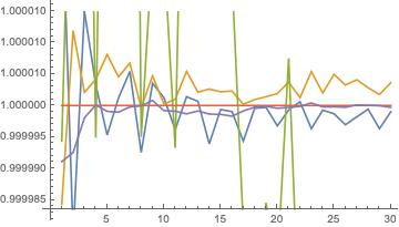
My test example concerned the estimation--in a 3D context--of nine values, four of which are known from prior considerations. (In the question, I stated three, but then realized that a fourth also is known.) The four values, one anticipates the quasirandom procedure will converge to are (see https://arxiv.org/abs/2004.06745) \begin{equation} \left\{\frac{1}{36},\frac{8 \pi }{27 \sqrt{3}},\frac{1}{81} \left(27+\sqrt{3} \log \left(97+56 \sqrt{3}\right)\right),\frac{2}{81} \left(4 \sqrt{3} \pi -21\right)\right\} \approx \end{equation} \begin{equation} \{0.027777777777777777778,0.53742203384717565944, 0.44597718463717723667, \ 0.018903515328657140917\}. \end{equation} In the estimation, I employed three billion 3D points, recording the results at intervals of one hundred million. A plot showing the four sets of results, along with the constant/target line 1, is

The yellow curve corresponds to the estimation of 0.44597718463717723667. The estimation of 0.02777777777777777777 is clearly the best of the four, hovering close to the constant line of 1. The blue curve corresponds to 0.53742203384717565944, while the (most highly fluctuating) green is for the smallest target value of 0.018903515328657140917.

These results were obtained using WorkingPrecision->20.

Then, due to my concerns, I undertook a repetition of the calculations, but now employing WorkingPrecision->40. After seven hundred million iterations, the results were identical to those obtained using WorkingPrecision->20. (Somewhat curiously, the computational time decreased by about $7\%$.) I am continuing to three billion iterations, as before, and will update this answer if I detect any deviations from the first set of results. Also, if there are no differences after the three billion, I will also note that.

But, as of now, it seems that the WorkingPrecision setting to 20 was certainly adequate for the task at hand.

Let me also note that as each quasirandom 3D point (Q1, Q2, Q3) is generated, I test to see if it satisfies the constraint \begin{equation} \text{Q1}>0\land \text{Q2}>0\land \text{Q3}>0\land \text{Q1}+3 \text{Q2}+2 \text{Q3}<1. \end{equation} If it does not, it is discarded from further consideration. Only $\frac{1}{36} \approx 0.027777777777777777778$ should satisfy the constraint (and as the plot shows, this is certainly the case).

UPDATE:

I now have two sets of results, both based on three billion iterations, the first having employed WorkingPrecision->20, the second, WorkingPrecision->40.

For each point (Q1,Q2,Q3) generated, I tested--as indicated above--whether it satisfied the constraint \begin{equation} \text{Q1}>0\land \text{Q2}>0\land \text{Q3}>0\land \text{Q1}+3 \text{Q2}+2 \text{Q3}<1. \end{equation} In both cases, the SAME number--83,333,308--of points passed the test, giving a probability of 0.0277777693333333, that is, very close to $\frac{1}{36}$, that a simple 3D integration yields.

Then, for each of these 83,333,308 points I tested whether it satisfied the further ("PPT"--"positive partial transpose") constraint \begin{equation} \text{Q1}^2+3 \text{Q1} \text{Q2}+(3 \text{Q2}+\text{Q3})^2<2 \text{Q1} \text{Q3}+3 \text{Q2}. \end{equation}

Now, the two number of points passing the further test were DIFFERENT, but almost identical. With WorkingPrecision->20, the number was 44,785,111 and with WorkingPrecision->40, it was two greater, that is, 44,785,113. (Let me note that the ratio [$R_1$] of the latter number to the common number 83,333,308, gives a further ratio [$R_2$] to the known value $\frac{8 \pi }{27 \sqrt{3}} \approx 0.53742203384718$ of 0.9999990427, closer to 1--as we would hope/expect--than the former [lesser WorkingPrecision] number of 44,785,111.)

I will now continue on my analyses with the higher setting of WorkingPrecision.