Beginner Simulating Gaussian Process with Correlation

Question

I have no little experience with algorithms. I would like to learn how to simulate a real valued Gaussian process with correlation (e.g., exponentially correlated $\Gamma(t)=e^{-\vert t \vert/2}).$

I've tried searching for such algorithms, but I cannot determine (i) how to simulate the process over the entire line instead of over some interval (using a Fourier transform) and (ii) how to give a discrete version of the algorithm.

Any examples or links to existing examples (perhaps with a minor explanation) would be extremely helpful.

Answer 1

I have not found any exemple of your problem but I used the Deserno text at https://www.cmu.edu/biolphys/deserno/pdf/corr_gaussian_random.pdf to code your problem as :

 cgrn = NestList[
   E^(-1/τ) # + 
     Sqrt[1 - (E^(-1/τ))^2] RandomReal[NormalDistribution[]] &, 
      RandomReal[NormalDistribution[]], 100];

As a beginner you certainly needs some explanations : Mathematica collects nearly all the programming paradigms but it is trully efficient if you use the functional programming one. So forget the loops. Here I use Nest --- more specifically NestList which insert in a list all the calculated elements of the nested function --- i.e. : $f[f[f[...[x]]...]$. Here one has $cgrn = [f[x], f^2[x],..., f^{100}[x]]$

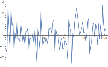
The best thing is not to list $cgrn$ but to plot it.

ListLinePlot[cgrn]

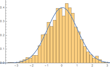
On must now verify if it is a gaussian process. As it is stationnary one can try to plot an histogram with more data --- 1000.

 ℋ = DistributionFitTest[cgrn, Automatic, "HypothesisTestData"];
 ℋ["TestDataTable", All]

If you know some thing about tests I let you find the result which can be verified by eyesight with

  Show[Histogram[cgrn, Automatic, "ProbabilityDensity"], 
  Plot[PDF[ℋ["FittedDistribution"], x], {x, -5, 5}, 
  PlotStyle -> Thick]]

Now in what concerns the autocorrelation function you have many choice to verify if it replicates what you expect.

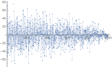
 acf = ListCorrelate[cgrn, cgrn, {1, 1}, 0];
 ListPlot[cgrn, Filling -> Axis]

or

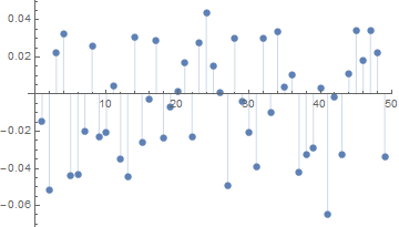
 ListPlot[CorrelationFunction[cgrn, {2, 50}], Filling -> Axis]

This last picture shows that I have made a mistake. I have tried also with the following code

 cgr[0] = RandomReal[NormalDistribution[]] ;
 cgr[n_] := cgr[n] = E^(-1/\[Tau]) cgr[n - 1] + Sqrt[1 - (E^(-1/\[Tau]))^2] RandomReal[NormalDistribution[]]
 cgrn1 := Table[cgr[i], {i, 1, 1000}];

but I encounter the same problem. Nevertheless I have decided to post my code since your question has no answer for a long time and perhaps it could help you. I hope also that an other person will see the code and will find my mistake.

I add tha of course I have not taken exactly your correlation function but even with a correction I encounter the same mistake.