Solving these system of 3 equations

Question

I have a function $f:\mathbb{R}^3\rightarrow \mathbb{R}^3$ and I'd like to find (numerically) roots of $f$.

My function f is the sum of two functions involving Solve, but the timing seems very reasonable, typically:

f[3, 6, 15.] // AbsoluteTiming
(* {0.002128, {-3., -6.83896, 12.6261}} *)

For the takers, f can be imported using

<< "http://pastebin.com/raw/uA9G2uYh" (* takes a few seconds *)

What I first tried but it takes too long (without returning errors)

FindRoot[f[x, y, z], {{x, 3}, {y, 5}, {z, 6}}] (* takes too long *)
NSolve[# == 0 & /. f[x, y, z] && 0 <= x <= 5 && 0 <= y <= 10 && 0 <= z <= 5]

It seems $f$ is linear in the first variable, so to simplify the problem, we can focus on:

g[t_, s_] := f[0, t, s][[2 ;;]]

Using Manipulate, I managed to identify some good initial conditions:

g[6.246, 18.725]
Plot[Evaluate@g[6.246, s], {s, 18.6, 18.8}]
(* {0.00204707, -0.00214908} *)

but still the following command never stops:

FindRoot[g[t, s], {{t, 6.246}, {s, 18.725}}]

Minimizing the norm of g also does not work (= never ends):

FindMinimum[Norm@g[t, s], {{t, 6.246}, {s, 18.725}}]

Question: How can I find the, or some, roots of g?

Answer 1

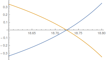
The equation f[x,y,z] does not lend itself well for finding roots.

I first tried to explore the space of the function, and got some error messages (stating that the equation could not be solved, etc).

n = 3;
A2 = {{0, 0, 0, 1, 0, 0}, {0, 0, 0, 0, 1, 0}, {0, 0, 0, 0, 0, 1}, {-2,
     1, 0, 0, 0, 0}, {1, -2, 1, 0, 0, 0}, {0, 0, -1, 0, 0, 0}};
lambda = {l1, 1, 1, l4, l5, 0};
ee[p_] := SparseArray[{{p, 1} -> 1, {6, 1} -> 0}] // Normal // Flatten
eqns1 = {(0.9786935821895908` a1 + 0.7848513153478486` a2 + 
        0.4355596199317594` a3) Cot[
       0.4450418679126288` t] + (-0.15544942857434468` a1 + 
        0.08626792451566725` a2 + 0.19384226684174244` a3) Cot[
       1.2469796037174667` t] + 
     0.30141660916782004` a2 Cot[1.8019377358048383` t] == 
    1 + (0.13414301076393745` a1 + 0.24171735309001358` a3) Cot[
       1.8019377358048383` t], (1.2204109352796038` a1 + 
        0.9786935821895927` a2 + 0.5431339622578357` a3) Cot[
       0.4450418679126288` t] + (0.28011019135741444` a1 - 
        0.15544942857434632` a2 - 0.3492916954160916` a3) Cot[
       1.2469796037174667` t] + (0.0596992560778067` a1 + 
        0.10757434232607628` a3) Cot[1.8019377358048383` t] == 
    1 + 0.13414301076393761` a2 Cot[1.8019377358048383` t], a1 == 0};
lambda1[tt_] := 
 Check[{a1, 1, 1, a2, a3, 0} /. Solve[eqns1 /. t -> tt] // Flatten, 
  Indeterminate]
eqns2 = # == 
     0 & /@ (MatrixExp[s*A2].(lambda + Inverse[A2].ee[2 n]) // 
      FullSimplify)[[n + 1 ;;]];
lambda2[ll1_, ss_] := 
 Check[({l1, 1, 1, l4, l5, 0} /. Solve[eqns2 /. s -> ss, {l4, l5}] // 
      N // Flatten) /. l1 -> ll1, Indeterminate]
f[l1_, t_, s_] := 
 f[l1, t, s] = 
  Check[(lambda1[t] - lambda2[l1, s])[[{1, 4, 5}]], Indeterminate]

    space = Table[{x, y, z} -> f[x, y, z], {x, 0, 5}, {y, 0, 10}, {z, 0, 
        5}];
    Extract[space, Position[space, Rule[a_, Indeterminate]]]


(*{{0, 0, 0} -> Indeterminate, {0, 0, 1} -> Indeterminate, {0, 0, 2} -> 
  Indeterminate, {0, 0, 3} -> Indeterminate, {0, 0, 4} -> 
  Indeterminate, {0, 0, 5} -> Indeterminate, {1, 0, 0} -> 
  Indeterminate, {1, 0, 1} -> Indeterminate, {1, 0, 2} -> 
  Indeterminate, {1, 0, 3} -> Indeterminate, {1, 0, 4} -> 
  Indeterminate, {1, 0, 5} -> Indeterminate, {2, 0, 0} -> 
  Indeterminate, {2, 0, 1} -> Indeterminate, {2, 0, 2} -> 
  Indeterminate, {2, 0, 3} -> Indeterminate, {2, 0, 4} -> 
  Indeterminate, {2, 0, 5} -> Indeterminate, {3, 0, 0} -> 
  Indeterminate, {3, 0, 1} -> Indeterminate, {3, 0, 2} -> 
  Indeterminate, {3, 0, 3} -> Indeterminate, {3, 0, 4} -> 
  Indeterminate, {3, 0, 5} -> Indeterminate, {4, 0, 0} -> 
  Indeterminate, {4, 0, 1} -> Indeterminate, {4, 0, 2} -> 
  Indeterminate, {4, 0, 3} -> Indeterminate, {4, 0, 4} -> 
  Indeterminate, {4, 0, 5} -> Indeterminate, {5, 0, 0} -> 
  Indeterminate, {5, 0, 1} -> Indeterminate, {5, 0, 2} -> 
  Indeterminate, {5, 0, 3} -> Indeterminate, {5, 0, 4} -> 
  Indeterminate, {5, 0, 5} -> Indeterminate}*)

f[x,0,z] is indeterminate.

Let's see how the function behaves in the rest of the space.

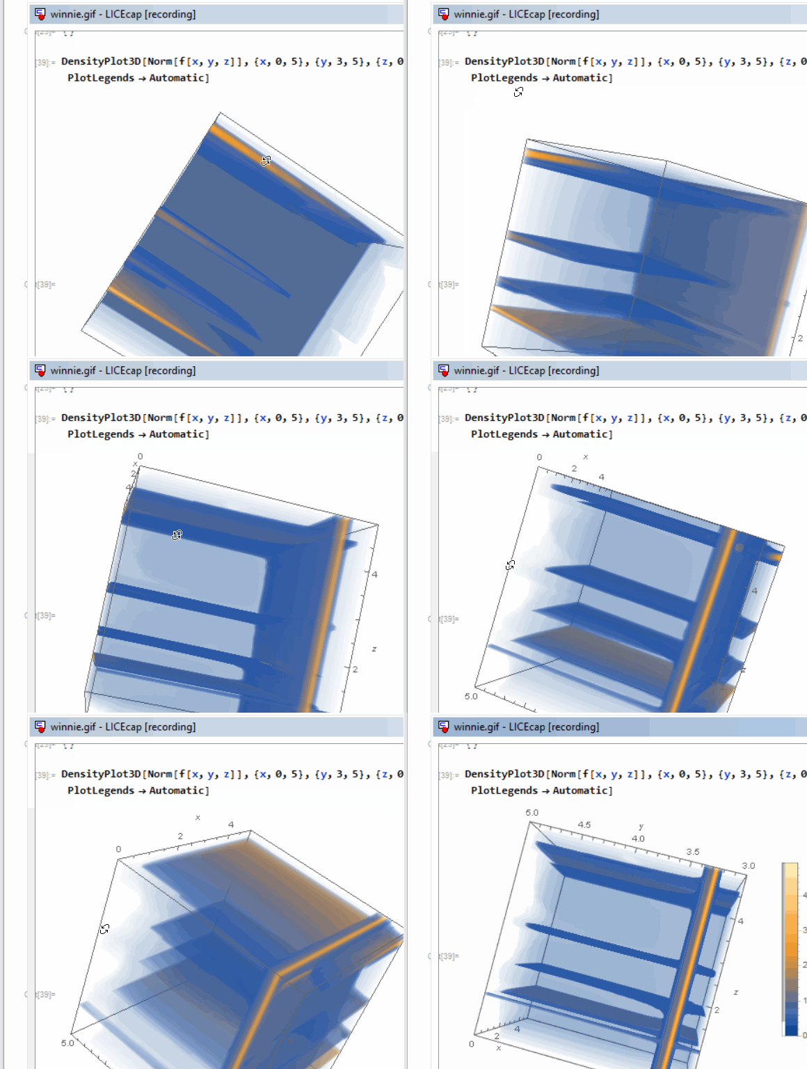
We can take the norm of the function. Zeros should be where the norm is zero.

DensityPlot3D[Norm[f[x, y, z]], {x, 0, 5}, {y, 3, 5}, {z, 0, 5}, 
 AxesLabel -> {x, y, z}, PlotLegends -> Automatic]

As you can see there are several planes of interest. You should focus on finding the roots within those ranges exclusively.