1
$\begingroup$

I am using Mathematica 10.0.2.0.

Here is the code I am working with:

    w[u_] = (-u*x^2*f[t, x] + 0.5*D[f[t, x], x, x]);

    wsol[u_] := 
      NDSolve[{D[f[t, x], t] == w[u], f[0, x] == 1, 
        f[t, -50] == Exp[-1000 t], f[t, 50] == Exp[-1000 t]}, 
       f, {t, 0, 100}, {x, -50, 50}, MaxStepSize -> 0.5, 
       AccuracyGoal -> 8, PrecisionGoal -> 8, 
       Method -> {"MethodOfLines", 
         "SpatialDiscretization" -> {"TensorProductGrid", 
           "MinPoints" -> 1000}}];

  wl[t] = Evaluate[
  Integrate[0.25*(x^2)*(f[t, x] /. wsol[0.25]), {x, -50, 50}]]

    Plot[Evaluate[wl[t]], {t, 0.01, 100}, PlotRange -> All]

Perhaps, I am doing something wrong but it takes a long time to plot, or sometimes does not plot at all.

Instead of plotting, I tried putting the data in a list but that took too long as well.

Additionally, I would like to fit a function to the data as well and measure the area under the curve.

I would really appreciate some help. Thanks.

$\endgroup$
6
  • $\begingroup$ do not integrate, do this process in NDSolve please. Try to make everything one more ' then the result will be the integration. $\endgroup$
    – Wjx
    Commented Jul 26, 2016 at 23:57
  • $\begingroup$ @Wjx I am not sure how to insert the $0.25*x^2$ inside NDSolve. $\endgroup$
    – Edv Beq
    Commented Jul 27, 2016 at 0:09
  • $\begingroup$ I also found a big mistake w[t] should be w[t_]; $\endgroup$
    – Edv Beq
    Commented Jul 27, 2016 at 0:24
  • $\begingroup$ Oh, then you can create another function and do the integration by D[newf[t,x],x]==0.25 x^2 f[t,x] $\endgroup$
    – Wjx
    Commented Jul 27, 2016 at 0:34
  • 1
    $\begingroup$ other issues aside, this code is repeatedly evaluating wsol with the same argument. Using memoization will help dramatically reference.wolfram.com/language/tutorial/… $\endgroup$
    – george2079
    Commented Jul 29, 2016 at 15:05

1 Answer 1

5
$\begingroup$

A quick solution with "SymbolicProcessing -> 0":

w[u_] = (-u*x^2*f[t, x] + 0.5*D[f[t, x], x, x]);

wsol[u_] := 
  NDSolve[{D[f[t, x], t] == w[u], f[0, x] == 1, f[t, -50] == Exp[-1000 t], 
    f[t, 50] == Exp[-1000 t]}, f, {t, 0, 100}, {x, -50, 50}];

core = f /. wsol[0.25][[1]]

wl[t_?NumericQ] := 
 NIntegrate[0.25*(x^2)*core[t, x], {x, -50, 50}, 
  Method -> {Automatic, "SymbolicProcessing" -> 0}, MaxRecursion -> 40]

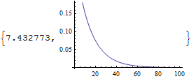
Plot[wl[t], {t, 0.01, 100}] // AbsoluteTiming

enter image description here

For more information you may want to read this post:

How to speed up the plot of NIntegrate?

$\endgroup$
2
  • 3
    $\begingroup$ +1 -- There seems to be quite a difference in wl[t] between the default 25-point x-grid and the 1001-point one of the OP or even a 101-point one. -- For merely plotting, one can usually speed things up a little more by lowering the precision goal in NIntegrate to PrecisionGoal -> 4 (but beware as it is lowered, the chance that the error estimator gets tricked seems to increase). $\endgroup$
    – Michael E2
    Commented Jul 29, 2016 at 14:01
  • $\begingroup$ Thank you, it is significantly faster even with high precision. Magic! $\endgroup$
    – Edv Beq
    Commented Jul 30, 2016 at 0:09

Your Answer

By clicking “Post Your Answer”, you agree to our terms of service and acknowledge you have read our privacy policy.

Not the answer you're looking for? Browse other questions tagged or ask your own question.