What is the difference between how Matlab and Mathematica solve State-Space and Transfer Function models?
I have a $16 \times 16$ state space system for which I am calculating transfer function. Mathematica and Matlab give me completely different answers. I can imagine truncation may lead to slightly different answers but what I get is a huge difference. I have checked the difference in numerical values to check the conditioning. There is no significant difference. I give the matrix as seen in Mathematica to you to check.
Please find the code attached!
a={{-(350103/48500), -14.9811, 0, 0, 0, 0, 0, 0, 0, 0, 0, 0, 0, 0, 0,
0}, {1.75898, -6.08528, 0, 0, 0, 0, 0, 0, 0, 0, 0, 0, 0, 0, 0,
0}, {0, 1, 0, 0, 0, 0, 0, 0, 0, 0, 0, 0, 0, 0, 0, 0}, {0, 0, 0, 0,
0, 0, 0, 0, 0, 0, 0, 0, 0, 0, 0, 0}, {12.4114, -32.0709, 310.284,
0, -19.63, -102.059, -310.284, 77.9757, 0, 0, 0, 0, 0, 0, 0,
0}, {2.21387, -5.72064, 55.3468, 0, -0.454893, -21.6178, -55.3468,
13.9089, 0, 0, 0, 0, 0, 0, 0, 0}, {0, 0, 0, 0, 0, 1, 0, 0, 0, 0, 0,
0, 0, 0, 0, 0}, {1, -2.584, 25, 0, -1, -7.016, -25, 0, 0, 0, 0, 0,
0, 0, 0, 0}, {0, 0, 0, 0, 12.4114, -32.0709, 310.284,
0, -19.63, -102.059, -310.284, 77.9757, 0, 0, 0, 0}, {0, 0, 0, 0,
2.21387, -5.72064, 55.3468, 0, -0.454893, -21.6178, -55.3468,
13.9089, 0, 0, 0, 0}, {0, 0, 0, 0, 0, 0, 0, 0, 0, 1, 0, 0, 0, 0, 0,
0}, {0, 0, 0, 0, 1, -2.584, 25, 0, -1, -7.016, -25, 0, 0, 0, 0,
0}, {0, 0, 0, 0, 0, 0, 0, 0, 12.4114, -32.0709, 310.284,
0, -19.63, -102.059, -310.284, 77.9757}, {0, 0, 0, 0, 0, 0, 0, 0,
2.21387, -5.72064, 55.3468, 0, -0.454893, -21.6178, -55.3468,
13.9089}, {0, 0, 0, 0, 0, 0, 0, 0, 0, 0, 0, 0, 0, 1, 0, 0}, {0, 0,
0, 0, 0, 0, 0, 0, 1, -2.584, 25, 0, -1, -7.016, -25, 0}};

b={{116319/1940}, {10.695}, {0}, {0}, {0}, {0}, {0}, {0}, {0}, {0},
{0}, {0}, {0}, {0}, {0}, {0}};

c={{0, 0, 0, 0, 0, 0, 0, 1, 0, 0, 0, 0, 0, 0, 0, 0}, {0, 0, 0, 0, 0, 0,
0, 0, 0, 0, 0, 1, 0, 0, 0, 0}, {0, 0, 0, 0, 0, 0, 0, 0, 0, 0, 0, 0,
0, 0, 0, 1}};

sys = StateSpaceModel[{a,b,c}]

BodePlot[sys, {2 \[Pi] 0.01, 2 \[Pi] 100},
ScalingFunctions -> {{Automatic, Automatic}, {Automatic, "Degree"}},
PhaseRange -> {-\[Pi], \[Pi]}, GridLines -> Automatic, ImageSize ->Large]
Corresponding Matlab code with the same set of matrices:
[num,den] = ss2tf(a,b,c,[0;0;0]);

P1 = tf(num(1,:),den);
P2 = tf(num(2,:),den);
P3 = tf(num(3,:),den);

figure; bode(P1,P2,P3);
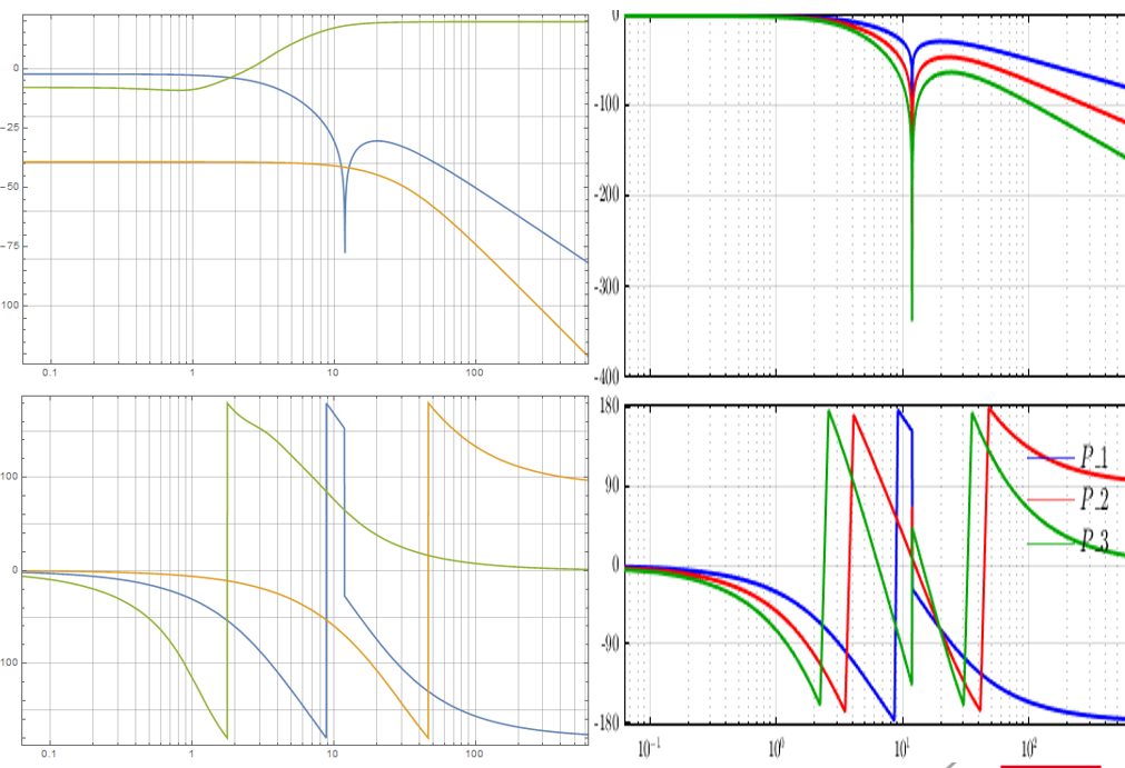
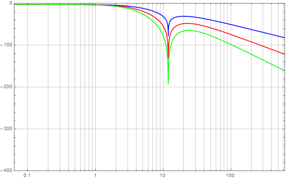
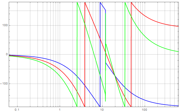
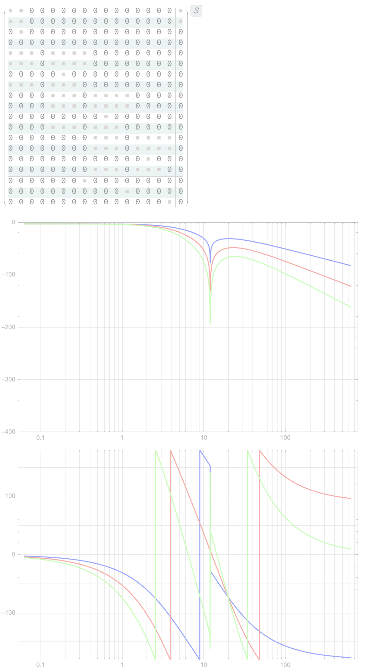
The transfer function that I can from Matlab and Mathematica are completely different in nature. I am pretty sure that according to theory Matlab gives me the right answer. But why is Mathematica so off the mark?
Could it be any of the following?
- Precision/truncation
- Size of the system
- Conditioning
Edit:
I have included the plots for both. Left is Mathematica and right is Matlab. The colors correspond to each other. Please take note of the Magnitude scale for both!

Any insight would be appreciated!


freq_rangewhich is undefined. Please include the full code in your question rather than the comments.) $\endgroup$CandDare reserved words in Mathematica and that the code given does not run because of that. One should avoid variable names with uppercase letters in Mathematica. After changing toa,b,c, anddthe code runs as advertised. $\endgroup$