1
$\begingroup$

I have a listplot and plot of fit functions which I combine with Show[listplot, plot]. However I also need to show the same plot with logarithmic axes. A proper way of doing this is avoiding any duplication of code, so that any changes on the legend, line style etc. always appears on both plots and doesn't need to be copied. How can this be done?

To make it more clear, my code looks like this:

 listplot=ListPlot[{data1, data2}, options1, option2, ...]
 plot=Plot[{f1[x], f2[x], ...}, {x,a,b}, options3, option4, ...]
 Show[listplot, plot]
$\endgroup$
3
  • $\begingroup$ I am not sure what you mean by avoiding the duplication of the code but how about LogLogPlot, ListLogLogPlot, they have the same options as Plot and ListPlot so you can assign the options beforehand and use the assignment. You can also set the options inside Show, however, I am not sure that this can contain all the options that are available for the Plot. $\endgroup$
    – atapaka
    Commented May 18, 2016 at 16:50
  • $\begingroup$ you can use ScalingFunctions. Chek this answer $\endgroup$
    – Sumit
    Commented May 18, 2016 at 17:04
  • $\begingroup$ @leosenko and Sumit I have made my question more explicit, but still don't know how to apply your suggestions without duplicating part of my code. $\endgroup$ Commented May 18, 2016 at 17:45

2 Answers 2

4
$\begingroup$

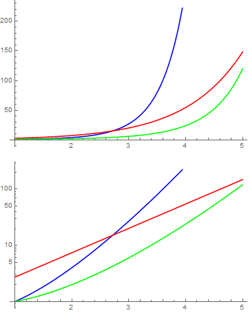
This should work, using a replacement rule to replace every y value with a scaled version, and then making sure that you have a scaled tick mark function as well

plot = Plot[{x^x, Exp[x], x!}, {x, 1, 5}, 
  PlotStyle -> {Blue, Red, Green}]
Show[plot /. Line[x__] :> (({#1, Log@#2} & @@@ x) // Line),
 PlotRange -> All,
 Ticks -> {Automatic, Charting`ScaledTicks[{Log, Exp}]}]

Mathematica graphics

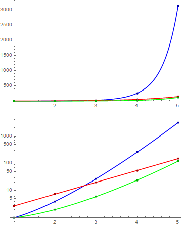
Or, with OP's example more explicitly

listplot = 
  ListPlot[Transpose[{#^#, Exp[#], #!} & /@ Range[1, 5]], 
   PlotStyle -> {Darker@Blue, Darker@Red, Darker@Green}];
plot = Plot[{x^x, Exp[x], x!}, {x, 1, 5}, 
   PlotStyle -> {Blue, Red, Green}, PlotRange -> All];
combined = Show[plot, listplot]
Show[combined /.
  {Line[x__] :> (({#1, Log@#2} & @@@ x) // Line), 
   Point[x__] :> (({#1, Log@#2} & @@@ x) // Point)},
 PlotRange -> All,
 Ticks -> {Automatic, Charting`ScaledTicks[{Log, Exp}]}]

Mathematica graphics

$\endgroup$
5
  • $\begingroup$ Any docs on Charting`ScaledTicks? $\endgroup$
    – BlacKow
    Commented May 18, 2016 at 20:45
  • $\begingroup$ It's one of those hidden functions I learned about from this site, like Charting`get2DPlotRange. I had to google it to find the example on here to follow. I do know it doesn't work as well on FrameTicks $\endgroup$
    – Jason B.
    Commented May 18, 2016 at 20:48
  • $\begingroup$ @BlacKow It seems like it should take two pure functions that are the inverse of each other, and scale accordingly, but I remember trying to do a simple example on a density plot with #^3 and #^(1/3) and not being able to get it to work. But it works for generating log ticks. Anything more complicated and I use the CustomTicks package's TickPreTransformation and TickPostTransformation functions $\endgroup$
    – Jason B.
    Commented May 18, 2016 at 21:07
  • $\begingroup$ I see... I was wondering why you need Exp and Log... Thank you! $\endgroup$
    – BlacKow
    Commented May 18, 2016 at 21:13
  • $\begingroup$ I tried Normal[plot] /. Line[x__] :> x to extract the coordinates of the plot, it failed. Did you know why? Other right trials I have done are Cases[plot, Line[x__] :> x, Infinity] or Reap@Plot[Sin[x], {x, -5, 5}, EvaluationMonitor :> Sow[{x, Sin[x]}]]. Thanks:) $\endgroup$
    – xyz
    Commented May 19, 2016 at 2:57
1
$\begingroup$

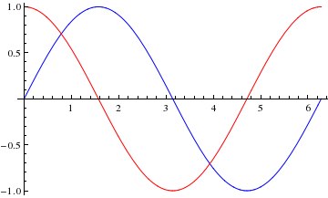
Lets say you already have this Plot.

f1[x_] := Sin[x]
f2[x_] := Cos[x]
plot1 = Plot[{f1[x], f2[x]}, {x, 0, 2 Pi}, PlotStyle -> {Blue, Red}]

enter image description here

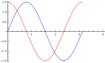
Now I am only going to change the scaling. I use a linear scaling. You can use Log as well

newplot[plot_, xmin_, xmax_, ymin_, ymax_] := Module[{fx, fy, q},
   fx[q_] := q/2;
   fy[q_] := 1.5 q;
   plot /. {Line[z__] :> Line[z /. {x_, y_} :> {fx[x], fy[y]}], 
   (PlotRange -> z__) :> PlotRange -> {{xmin, xmax}, {ymin, ymax}}}]

You must define new PlotRange as xmin, xmax, ymin, ymax, otherwise the plot may not look good. And Now we apply it on our existing plot

newplot[plot1, 0, 4, -1.5, 1.5]

enter image description here

New scaling with old options. If you want to convert the x values with their Log use fx[q_]:=Log[q] and likewise..

$\endgroup$

Your Answer

By clicking “Post Your Answer”, you agree to our terms of service and acknowledge you have read our privacy policy.

Not the answer you're looking for? Browse other questions tagged or ask your own question.