How to add data to an existing plot?

Question

Sometimes I need to plot functions that take quite a while to calculate--and sometimes I need to replot in light of what I see on the plot. Is it possible to add points to a plot one by one, as they are calculated, so that I can preview how its coming out?

In the code below, I calculate a function at 240 values of x. If I replot after every point, I'll end up with a series of 240 plots, which is not what I want. Is it possible to just draw one plot and add the newly-calculated points to it?

z[n_, x_] := Nest[#^2 + x &, x, n];
center = -1.40115518909205`60;
side = N[(3*10^-15), 60];
steps = 120;
stepSize = side/steps;
a = Table[z[-1 + 2^28, center + n*stepSize], {n, -steps, steps}];
ListPlot[a, PlotStyle -> PointSize[Small], DataRange -> {-side, side}]

(If anyone has some tips on speeding this calculation up, that would also be appreciated.)

Answer 1

If you wanted to only ever have one plot the two ways come to mind. One is similar to @bbgodfrey's method but incorporating some front end code to delete the previous plot. The other is to make the plot dynamic:

a = Table[n, {n, -20, 20}];
Dynamic[ListPlot[a, DataRange -> {-1, 1}], TrackedSymbols :> {a}]

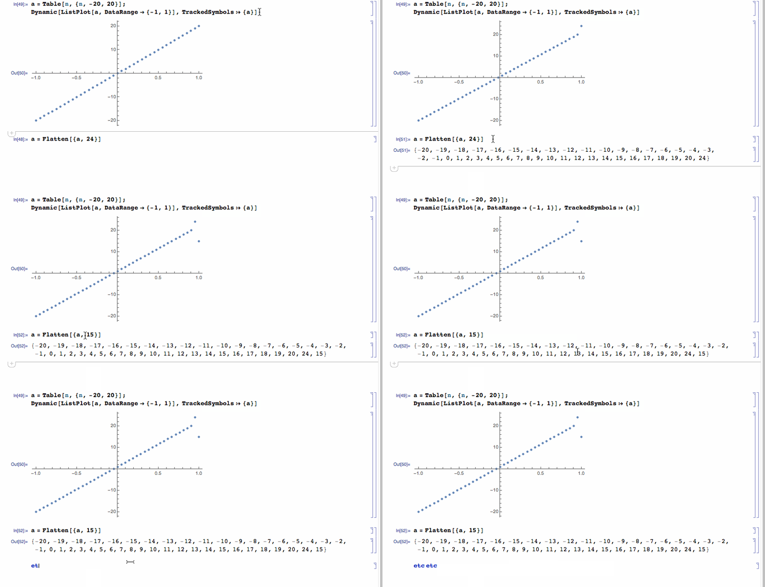
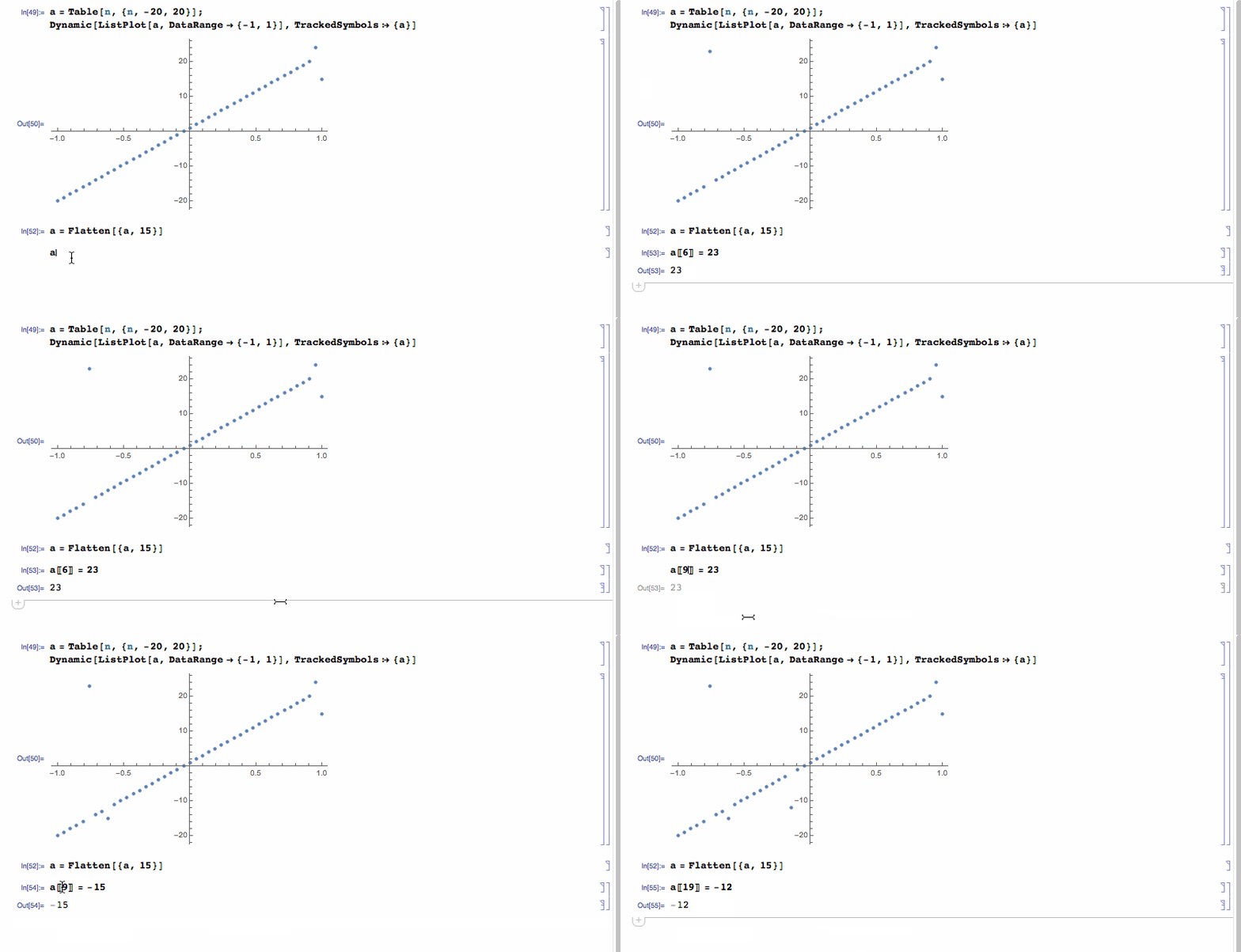
Now every time you change a the plot will change. The example below is quick and dirty. I've used Flatten to modify a but there are many other ways: Join, Append, Prepend and so on.

Edit

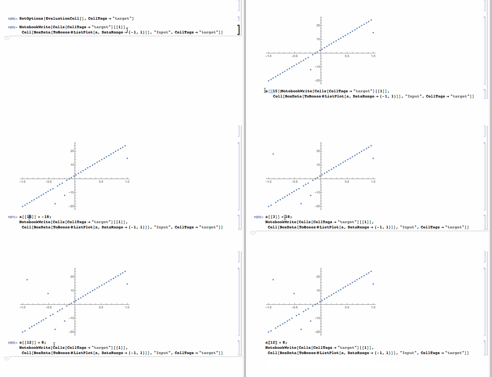
there are a few ways to do it without using dynamic. Here is a reference to something @Kuba posted:

SetOptions[EvaluationCell[], CellTags -> "target"]

then

NotebookWrite[Cells[CellTags -> "target"][[1]], 
 Cell[BoxData[ToBoxes@ListPlot[a, DataRange -> {-1, 1}]], "Input", 
  CellTags -> "target"]]

Answer 2

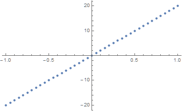
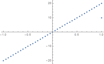
I take it that you wish to add points to an existing plot without using Show. Consider the toy problem,

a = Table[n, {n, -20, 20}];
plt = ListPlot[a, DataRange -> {-1, 1}]

To add

newpoint = {1, 10}

do the following.

pts = Join[Catenate@Cases[plt, Point[z_] -> z, Infinity], {newpoint}];
plt /. Point[_] -> Point[pts]

which contains the new point, as desired. Additional points can be added by Joining or Appending them to pts.

Addendum

To have only one Plot displayed in the notebook, use

a = Table[n, {n, -20, 20}];
plt = ListPlot[a, DataRange -> {-1, 1}];
Dynamic[plt]

which displays the first plot above. Then

newpoint = {1, 10};
plt = plt /. Point[z_] :> Point[Append[z, newpoint]];

will cause the first plot to be replaced by the second.

Answer 3

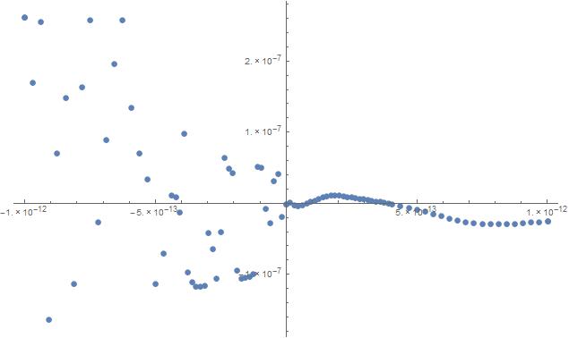
From the OP: This is just a demo of the Dynamic[] method Mike recommended above. This is exactly the effect I wanted to create for when I'm looking at a bifurcation point of a slooow calculation.

(* Function and endpoints *)
z[n_, c_] := Nest[#^2 + c &, c, n];
center = -1.40115518909205`60;
delta = N[(1*10^-12), 60];
r=22;
f[x_] := z[-1 + 2^r, center + x];


(*This array t makes the data pts fill in from the centre out, in layers*)
t = Flatten[{-1, 1, 0, Table[Table[{-i, i}, {i, 1, -1 + 2^j, 2}]/(2^j), {j, 1, 6}]}];

(* Initialize the plot with the first, middle, last points *)
fml = delta*{-1, 0, 1} ; a = Transpose[{fml, f[fml]}];
Dynamic[ListPlot[a, DataRange -> {-delta, delta}], TrackedSymbols :> {a}]
Do[
    x = t[[i]]*delta;
    AppendTo[a, {x, f[x]}], {i, 1, Length[t]}]

Give it a few seconds, because it's slow (which was the point of all this), and depending on how you change the parameters the initial plot might not plot because of values of f[x] with no sig figs. If it's too slow on your computer, decrease r a bit. Sorry, I don't know how to create/upload a cool animation like Mike did.