13
$\begingroup$

A unit distance graph is a graph that is embeddable in the plane so that every edge has length 1.

UnitDistanceQ[input_]:=Module[
    {g, x, F, v, min, nod, gl},
    g = input;
    gl = Length[g]; (* Vertex Count *)
    (* 2 vertex count variables x1, x2, etc... *)
    x = Table[Symbol@@ToExpression["x" <> ToString[i]], {i, 1, 2*gl}]; 
    (* The force to minimize is the squared error of the lengths *) 
    F = \!\(
\*UnderoverscriptBox[\(\[Sum]\), \(i = 1\), \(gl\)]\(
\*UnderoverscriptBox[\(\[Sum]\), \(j = 1\), \(gl\)]g[[i, j]] \((\((x[[2  i]] - x[[2  j]])\)^2 + \((x[[2  i - 1]] - x[[2  j - 1]])\)^2 - 1)\)^2\)\);
    (* Initial vertex positions *)  
    v = Table[gl*Random[], {i, 1, 2*gl}];
    (* Minimization *)  
    {min, nod} = FindMinimum[F, Transpose[{x,v}], Method->"QuasiNewton"];
    (* Output Solution *)       
    If[min < 10^-3,
        Print[{min,nod}];
        GraphPlot[g, VertexCoordinateRules -> 
            Thread[Range[gl] -> Partition[ x /. nod, 2]],
        AspectRatio -> Automatic, 
        VertexLabeling -> None, 
        ImageSize->Small]
    ]
]

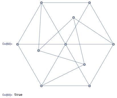
For example, the Golomb graph is unit distance.

 g = Graph[
          UndirectedEdge @@@ {{1, 2}, {1, 3}, {1, 4}, {2, 3}, {2, 6}, {3, 
             8}, {4, 5}, {4, 9}, {4, 10}, {5, 6}, {5, 10}, {6, 7}, {6, 
             10}, {7, 8}, {7, 10}, {8, 9}, {8, 10}, {9, 10}}];
    m = AdjacencyMatrix[g];
    UnitDistanceQ[m]
    (* gives
        FindMinimum::sdprec: Line search unable 
             to find a sufficient decrease in the function value with 
             MachinePrecision digit precision. >> 
*)

So the question is how to check for a unit distance embedding as fast as possible, my code is not working yet but I think something along these lines will work...

My iterative approach works well for the Golomb graph when run many times
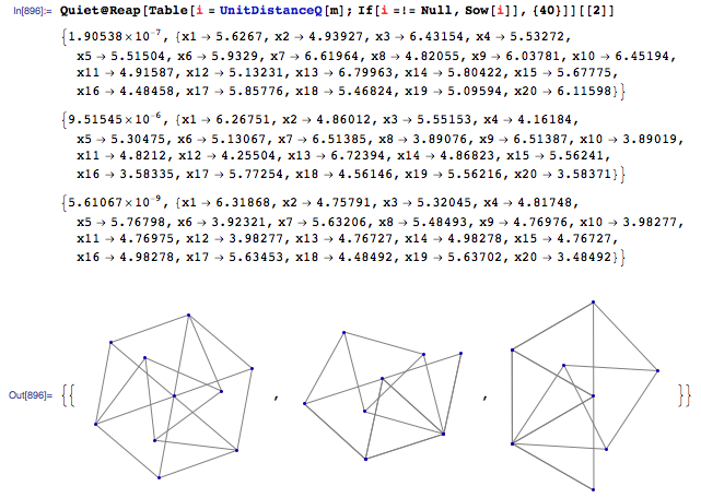
enter image description here

This is a great question and cool algorithms could be invented here!

$\endgroup$
7
  • $\begingroup$ Would you kindly explain how the function UnitDistance is meant to work? $\endgroup$
    – DavidC
    Commented Aug 27, 2012 at 22:52
  • $\begingroup$ It lays out a graph with random vertex positions and then iteratively moves them to decrease the energy functional F which makes every edge become unit distance for instance: Quiet@Reap[ Table[i = UnitDistanceQ[m]; If[i =!= Null, Sow[i]], {100}]][[2]] $\endgroup$
    – M.R.
    Commented Aug 27, 2012 at 22:59
  • $\begingroup$ Thanks for the explanation. Interesting approach. Btw, if g is a graph, you'll want to use VertexCount rather than Length to determine the number of vertices. $\endgroup$
    – DavidC
    Commented Aug 27, 2012 at 23:02
  • $\begingroup$ In my code g is the adj matrix, bad name i guess. $\endgroup$
    – M.R.
    Commented Aug 27, 2012 at 23:08
  • $\begingroup$ Ok. That clarifies things. $\endgroup$
    – DavidC
    Commented Aug 27, 2012 at 23:11

4 Answers 4

7
$\begingroup$

Basically along the lines suggested by Bill Simpson. The equation setup could perhaps be done with more elegance. Still, it's fairly short code.

isUnitDistance[graph_] := Module[
  {verts, edges, n, coords, p, x, soln},
  verts = VertexList[graph];
  edges = EdgeList[graph];
  n = Length[verts];
  verts = verts /. Thread[verts -> Range[n]];
  coords = Array[x, {n, 2}];
  {x[1, 1], x[1, 2], x[2, 1], x[2, 2]} = {0, 0, 1, 0};
  p[j_] := {x[j, 1], x[j, 2]};
  polys = 
   Map[(p[#[[1]]] - p[#[[2]]]).(p[#[[1]]] - p[#[[2]]]) - 1 &, edges];
  Quiet[soln = NSolve[polys]];
  If[soln === {}, False, True]
  ]

For run time, don't expect miracles. More than a very few vertices and it could go into overtime.

SeedRandom[111111];
gg = Graph@
  Union[Sort /@ (RandomInteger[{1, 8}, {20, 2}] /. {j_, j_} :> 
       Sequence[])]

(Still running after 2+ minutes.)

Could try to do similarly using NMinimize on sums of squares of distances minus 1. That's just a heuristic though, and a failure to attain a positive result is not a strong indication that no such solution exists.

$\endgroup$
3
  • $\begingroup$ Running my original function many times works much faster than this: Quiet@Reap[ Table[i = UnitDistanceQ[m]; If[i =!= Null, Sow[i]], {100}]][[2]] However the coordinates are not exact solutions, is there a way to rederive them? $\endgroup$
    – M.R.
    Commented Aug 28, 2012 at 3:37
  • $\begingroup$ I prefer the iterative method because of speed but also because you can see the local minima as interesting embeddings in themselves. $\endgroup$
    – M.R.
    Commented Aug 28, 2012 at 3:41
  • $\begingroup$ Why not use RandomGraph? $\endgroup$ Commented Oct 25, 2014 at 21:34
2
$\begingroup$

I do not know how to compute whether a graph is a unit distance graph.

However, if you know the name of a graph you can ask Mathematica directly. For example,

GraphData["GolombGraph"]
GraphData["GolombGraph", "UnitDistance"]

golomb

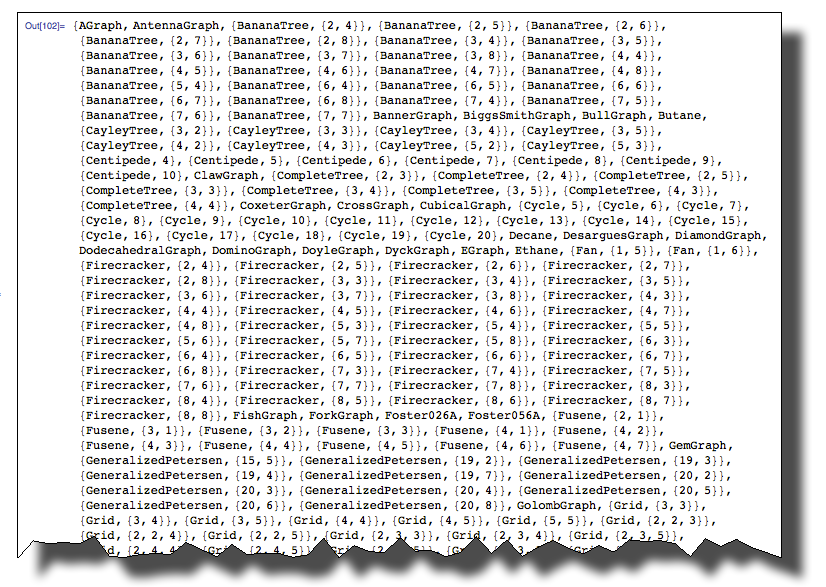
As you may know, graphs that Mathematica classifies as unit distance graphs are the following:

Cases[{#, GraphData[#, "UnitDistance"]} & /@ GraphData[], {g_, True} :> g]
Length@%

unit distance graphs

454

$\endgroup$
2
  • 1
    $\begingroup$ I know about GraphData and it is a nice repository, but does not answer the question. $\endgroup$
    – M.R.
    Commented Aug 27, 2012 at 22:01
  • $\begingroup$ Yeah, I think maybe that only works for graphs that are already "known" to be unit distance. Maybe I'm wrong? $\endgroup$ Commented Oct 25, 2014 at 16:34
2
$\begingroup$

If your graph is not one of the ones known to Mathematica then this might help.

e = {(x1 - x2)^2 + (y1 - y2)^2 == 1, (x1 - x3)^2 + (y1 - y3)^2 == 1,
     (x1 - x4)^2 + (y1 - y4)^2 == 1, (x2 - x3)^2 + (y2 - y3)^2 == 1,
     (x4 - x5)^2 + (y4 - y5)^2 == 1, (x5 - x6)^2 + (y5 - y6)^2 == 1,
     (x6 - x7)^2 + (y6 - y7)^2 == 1, (x7 - x8)^2 + (y7 - y8)^2 == 1,
     (x8 - x9)^2 + (y8 - y9)^2 == 1, (x9 -x10)^2 + (y9 -y10)^2 == 1, 
     x1 == 0, y1 == 0, x2 == 1, y2 == 0};
Reduce[e, {x1,y1,x2,y2,x3,y3,x4,y4,x5,y5,x6,y6,x7,y7,x8,y8,x9,y9,x10,y10}]

That pins a couple of points to the paper and very rapidly determines and returns a couple of choices for positions of some of your subsequent points. You could use that result to fairly quickly determine if there are no satisfactory positions for the rest of your points. Choice of which equations to include has a significant effect on the speed of finding solutions. Sometimes adding an equation will speed it up, others will substantially slow it down. I don't know if you wait long enough whether it would find a solution for all your points.

$\endgroup$
1
  • $\begingroup$ This is a nice approach, but I'm trying want a general approximation algorithm: a function to run on any and all graphs. $\endgroup$
    – M.R.
    Commented Aug 27, 2012 at 23:01
2
$\begingroup$

Simulated annealing will get an algorithm that works the way you want... but will require more careful guidance / tweaking / adaptive adjustment than what I include below:

Meas[G_, i_: 0] := Module[{
 Ex = EdgeList[G],
 P = N[PropertyValue[{G, #}, VertexCoordinates] & /@ VertexList[G]]
},
Return[If[i == 0,
 Max[Abs[
  Map[Norm[#[[1]] - #[[2]]] &, 
   Map[P[[#]] &, Map[List @@ # &, Ex], 1], 1] - 1]],
  Max[Abs[
   Map[Norm[#[[1]] - #[[2]]] &, Map[P[[#]] &, Map[List @@ # &,
       Select[Ex, MemberQ[#, i] &]
       ], 1], 1] - 1]]
 ]]
];

STEP[G_, \[Epsilon]_: 0.05, \[Delta]_: 0.1] := Module[{
 Vx = VertexList[G],
 Ex = EdgeList[G],
 n, m, P, i, G2, P2
 },
n = Length[Vx]; m = Length[Ex];
P = PropertyValue[{G, #}, VertexCoordinates] & /@ Vx;
P2 = P;
i = RandomInteger[{1, n}];
P2[[i]] = P2[[i]] + \[Delta] ({RandomReal[], RandomReal[]} - 0.5);
G2 = Graph[Vx, Ex, VertexCoordinates -> P2];
If[Meas[G2, i] < Meas[G, i] || RandomReal[] < \[Epsilon], Return[G2], Return[G]
]]

Unfortunately this won't really work well without some more careful application than using a constant epsilon, delta, Meas. It's a random algorithm, it's not necessarily going to work at all, but even so this is a tricky problem. A random graph isn't likely to work, but even then you can see it in action doing, well, something:

G = RandomGraph[{15, 20}];
P = Table[{RandomReal[], RandomReal[]}, {q, 1, Length[VertexList[G]]}];
G = Graph[G, VertexCoordinates -> P];
DATA = NestList[STEP, G, 5000];
Manipulate[DATA[[i]], {i, 1, Length[DATA], 1}]

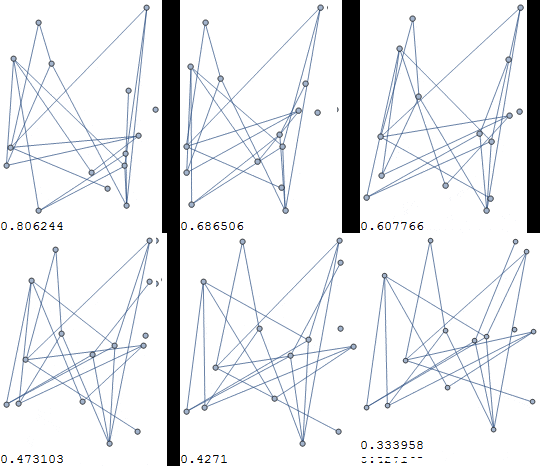
Short term:

short-term animation

Long term:

long-term animation

What is nice is you might see some small unit graphs bouncing around inside the larger graph as you go.

It doesn't even work optimally with a known unit graph:

G = GraphData["GolombGraph"];
P = Table[{RandomReal[], RandomReal[]}, {q, 1, Length[VertexList[G]]}];
G = Graph[VertexList[G], EdgeList[G], VertexCoordinates -> P];
DATA = NestList[STEP[#, 0.01, 0.2] &, G, 500000];
Animate[ColumnForm[{DATA[[i]], Meas[DATA[[i]]]}], {i, 1, Length[DATA],1}]

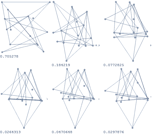
Short term:

short-term animation

Long term:

long-term animation

(Sorry for the artifacts, I had to compress it way too much with some web tool to make it small enough, and so it's a bit tweaked.)

In addition to changing parameters like epsilon and delta, you can adjust the Meas metric to be some Lp norm, max, average, whatever you like.

$\endgroup$

Your Answer

By clicking “Post Your Answer”, you agree to our terms of service and acknowledge you have read our privacy policy.

Not the answer you're looking for? Browse other questions tagged or ask your own question.