Is it possible to extract data from an EPS plot not generated in Mathematica?

Question

I want to extract data from an EPS plot not generated in Mathematica and replot it. In general is it possible to extract data from plots in any formats in Mathematica? I searched but unfortunately didn't find the answer.

As an example extracting the coordinates of the following plots:

The EPS file is here.

Answer 1

Mathematica can Import your file, and the result is a handy set of graphical primitives. So in this particular case we can do all the steps needed for data extraction without leaving Mathematica. I will not do the whole work for you but show the correct approach to the problem.

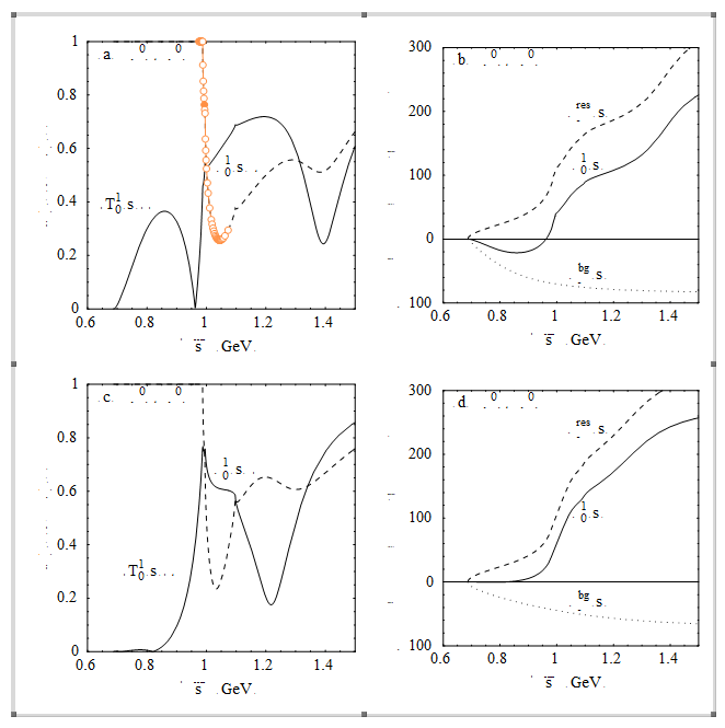
First, you Import the file and check in what form the curves of interest are present in the imported figure. For this purpose you double-click on a curve:

fig = Import["http://pastebin.com/raw.php?i=di8Abah4", "EPS"]

From the screenshot it is seen that selected dashed line is continuous, what is the best situation for you. (In many cases dashed (and even solid on-screen) lines are represented by a collection of two-point line segments which are harder to deal with.)

At the next step you inspect its internal structure. For this purpose I recommend my shortInputForm function:

fig // shortInputForm

From the output you can see that all the textual elements are present in the form Style[{___Text}, ___] and all the lines are encoded as JoinedCurves. At this step you remove all the textual elements, decode JoinedCurves using undocumented GeometricFunctions`DecodeJoinedCurve and show the frame at the same time:

cleanFig = 
 Show[fig /. {Style[{___Text}, ___] :> (## &[]), 
    c_JoinedCurve :> GeometricFunctions`DecodeJoinedCurve@c}, 
  Frame -> True]

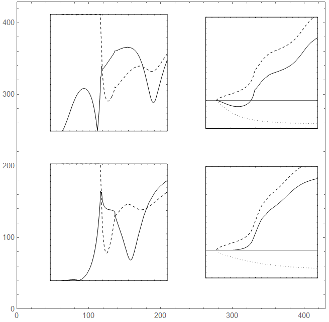
After this the internal structure of the figure becomes much more clear:

fig // shortInputForm

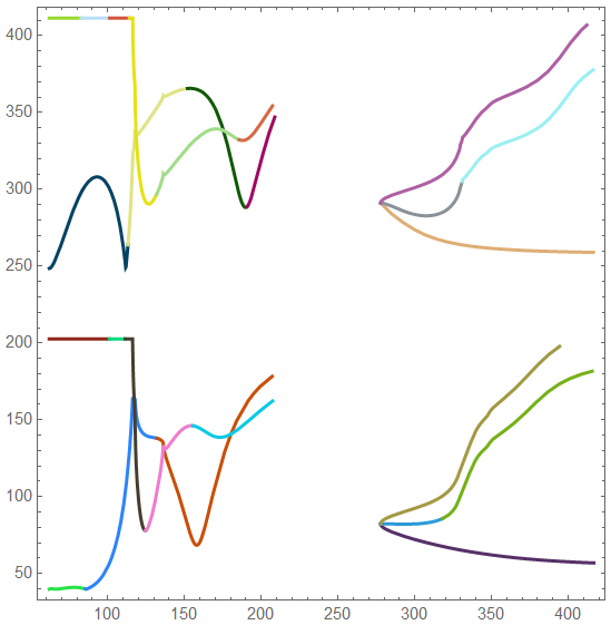
From this output you see that the mutipoint curves are represented by the structures of the form JoinedCurve[{{__Line}}, ___] with more than 2 Line primitives. Extracting them as sets of points and plotting again with random colors and indexes attached as Tooltips:

multipointCurves = 
  Cases[cleanFig, 
   JoinedCurve[{points : {__Line} /; Length[points] > 2}, ___] :> 
    Level[points, {-2}], Infinity];
Graphics[MapIndexed[Tooltip[{Thick, RandomColor[], Line[#]}, #2] &, 
  multipointCurves], Frame -> True]

Now from the figure you can easily find the index of each line from the tooltip and then extract its points by the index from multipointCurves. For example, the top left line consists from 6 fragments with indices {17, 18, 19, 20, 21, 22}, so the whole curve can be extracted as multipointCurves[[{17, 18, 19, 20, 21, 22}]].

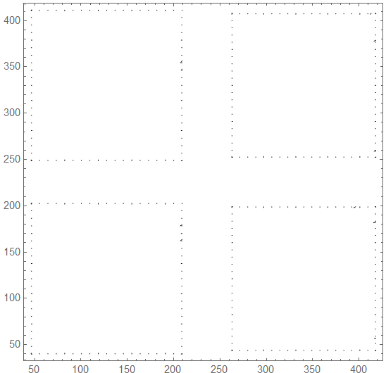
At this point we finish with curves and need to find the correspondence between the coordinate system of the figure and the internal coordinate system of each of the plots shown on the figure. For this purpose we should extract all the ticks which are encoded as JoinedCurve[{{Line[{{_Real, _Real}, {_Real, _Real}}]}}, ___] where Line has length knowingly lesser than 10 (as seen thanks to the Frame):

allTicks = 
  Cases[cleanFig, 
   JoinedCurve[{{l : 
         Line[{a : {_Real, _Real}, b : {_Real, _Real}}]}} /; 
      Norm[a - b] < 10, ___] :> l, Infinity];
Graphics[allTicks, Frame -> True]

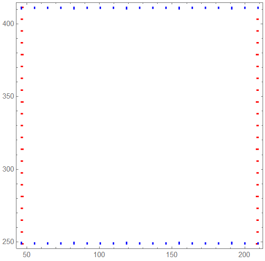
Now we concentrate on the upper left plot in the figure. We note that all its ticks have coordinates in the PlotRange -> {{0, 220}, {240, 420}}. And horizontal ticks have equal $y$-coordinates of both points, while vertical ticks have equal $x$ coordinates:

upperLeftTicksVertical = 
  Cases[allTicks, 
   Line[{{ax_, ay_}, {bx_, by_}}] /; 
    ax == bx < 220 && ay > 240 && by > 240];
upperLeftTicksHorizontal = 
  Cases[allTicks, 
   Line[{{ax_, ay_}, {bx_, by_}}] /; 
    ax < 220 && bx < 220 && ay == by > 240];
Graphics[{Thick, Blue, upperLeftTicksVertical, Red, 
  upperLeftTicksHorizontal}, Frame -> True]

Now we can check how precisely ticks are positioned, for example checking only the first horizontal coordinates of the vertical ticks (output is truncated):

Differences@Sort@upperLeftTicksVertical[[;; , 1, 1, 1]]

{0.`, 9.048700737450702`, 0.`, 9.04707210160884`, 0.`, 
9.048700737450702`, 0.`, 9.047072101608833`, 0.`, 9.048700737450758`, 
0.`, 9.047072101608805`, 0.`, 9.048700737450716`,

We see that the precision is very good but not ideal. From my experience, in the most practical cases the precision is MUCH worse and some regression analysis is needed in order to minimize the recovery error.

Now we need to establish the correspondence between ticks and their actual meanings. From the original figure we find that the vertical ticks in the left upper plot go from 0.6 to 1.5 with step 0.05. So we can fit the linear model where the independent variable is the actual meaning of the tick (which has no error) and the response is its coordinate on the figure (which is noisy):

upperLeftTVFit = 
 LinearModelFit[
  Transpose[{Sort[Range[.6, 1.5, .05]~Join~Range[.6, 1.5, .05]], 
    Sort[upperLeftTicksVertical[[;; , 1, 1, 1]]]}], x, x];

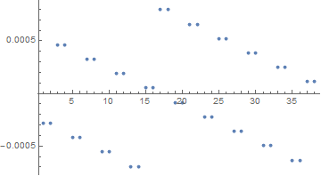
Let us see on the fit residuals:

ListPlot[upperLeftTVFit["FitResiduals"], PlotRange -> All]

Looks like a rounding off error as it should.

Now we need to take the inverse of this function in order to be able to convert the figure coordinates into the internal coordinates of the plot:

upperLeftXConvert = InverseFunction[upperLeftTVFit["Function"]]

0.00552611 (62.339 + 1. #1) &

When repeating this procedure for the horizontal ticks we take into account that for some reason the upper right tick is absent:

upperLeftTHFit = 
  LinearModelFit[
   Transpose[{Sort[Range[0, 1, .05]~Join~Range[0, .95, .05]], 
     Sort[upperLeftTicksHorizontal[[;; , 1, 1, 2]]]}], x, x];
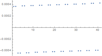
ListPlot[upperLeftTHFit["FitResiduals"], PlotRange -> All]
upperLeftYConvert = InverseFunction[upperLeftTHFit["Function"]]

0.00614072 (-248.648 + 1. #1) &

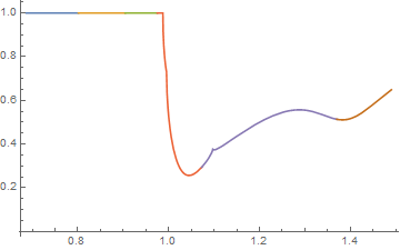
Now we can plot the first curve in its natural coordinate system:

ListLinePlot[
 multipointCurves[[{17, 18, 19, 20, 21, 22}]] /. {x_Real, 
    y_Real} :> {upperLeftXConvert[x], upperLeftYConvert[y]}]

Voilà!