17
$\begingroup$

Michael E2 wrote a wonderful solution for my question. Now I am considering the system:

$$ \begin{align*} x'&=x^2 y,\ x(0)=1\\ y'&=-x y^2,\ y(0)=1 \end{align*} $$

I am wondering how I can write this in vector form to produce a solution $\vec r(t)$ directly using NDSolve like Michael did.

Edits due to Suggestions: Daniel Lichtblau suggested:

f[vals : {_?NumberQ ..}] := {vals[[1]]^2*vals[[2]], -vals[[1]]* vals[[2]]^2};
vsoln = NDSolveValue[{x'[t] == f[x[t]], x[0] == {1, 1}},  x[t], {t, 0, 1}];
ParametricPlot[vsoln, {t, 0, 1}]

Which produces this plot.
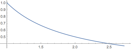
enter image description here

And here is Michael E2 suggestion:

f[{x_, y_}] := {x^2*y, -x*y^2};
vsoln = NDSolveValue[{x'[t] == f[x[t]], x[0] == {1, 1}}, x, {t, 0, 1}];
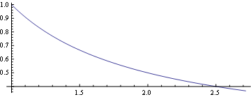
ParametricPlot[vsoln[t], {t, 0, 1}]

Which produces the same plot.

This is absolutely amazing that this works. NDSolveValue interprets x'[t] == f[x[t]] as {x'[t],y'[t]}==f[x[t],y[t]] because of x[0]=={1,1} ? Wow! What is going on here?

$\endgroup$
5
  • $\begingroup$ In general it will be hard to mimic my other answer. The equations of the system have to have a form that is amenable. Daniel's answer below is easier to generalize and understand. (However, a solution for the present case is possible: NDSolve[{r'[t] == ({{0, 1}, {-1, 0}}.r[t]) r[t]^2, r[0] == {1, 1}}, r, {t, 0, 1}].) $\endgroup$
    – Michael E2
    Commented Mar 31, 2015 at 3:38
  • 2
    $\begingroup$ It's a vectorial interpretation of the dependent variable. Documented, actually. Just sometimes frustrating to get working if the ode is nonlinear. $\endgroup$ Commented Mar 31, 2015 at 19:43
  • $\begingroup$ @DanielLichtblau Ah! Documented? I've been looking for this in the documentation. Could you point me toward an example of this in any documentation? $\endgroup$
    – David
    Commented Apr 1, 2015 at 15:38
  • 1
    $\begingroup$ Help > Documentation Center > NDSolve > Examples > Scope > Ordinary Differential Equations > "Solve for a vector-valued function:". To answer the next question, yes, I really did drill down that far to find out how to do this. Also there is an example "Use matrix-valued variables to compute the fundamental matrix solution:" $\endgroup$ Commented Apr 1, 2015 at 15:47
  • $\begingroup$ Aha! Deduced from the initial condition! But I don't see an example like this: f[{x_, y_}] := {x^2*y, -x*y^2}; vsoln = NDSolveValue[{x'[t] == f[x[t]], x[0] == {1, 1}}, x, {t, 0, 1}]; ParametricPlot[vsoln[t], {t, 0, 1}], $\endgroup$
    – David
    Commented Apr 2, 2015 at 4:14

3 Answers 3

13
$\begingroup$

Something like this? Make the rhs a "black box" so it does not show explicit dimenions. Use it in NDSolve.

f[vals : {_?NumberQ ..}] := {vals[[1]]^2*vals[[2]], -vals[[1]]*
   vals[[2]]^2}

vsoln = 
 NDSolveValue[{x'[t] == f[x[t]], x[0] == {1, 1}}, x[t], {t, 0, 1}]


(* Out[275]= InterpolatingFunction[{{0., 1.}}, <>][t] *)

Obviously that black box will be about as complicated as was the original rhs. No free lunch on that account.

$\endgroup$
7
  • $\begingroup$ Amazing! But I do need some help. The notation f[vals: {_?Number Q ..}]. That I don't understand. First, the colon, what does that mean. Then I think the ?NumberQ is just asking if something is a number, but the underline before and the dots after, what do they mean? Where can I read more examples of this type of thing? $\endgroup$
    – David
    Commented Mar 30, 2015 at 21:39
  • $\begingroup$ The colon is a way of giving the pattern that follows it a name (in this case, vals). That's so it can be used on the right side of the SetDelayed. The ?NumberQ (no space before Q) is a predicate test; if the input is not an explicit number then the pattern does not match. The .. makes it into a "repeated" form of the pattern; it will match one or more NumberQ items. A good place to read up on this might be the documentation e.g. for NDSolve, since there are a good number of examples therein. Not sure any show quite this approach but maybe some are similar. $\endgroup$ Commented Mar 30, 2015 at 22:42
  • $\begingroup$ I might define f in terms of the system: f[{x_, y_}] := {x^2*y, -x*y^2}, with or without a PatternTest. (+1) $\endgroup$
    – Michael E2
    Commented Mar 31, 2015 at 3:34
  • $\begingroup$ @MichaelE2 I am not sure I follow your suggestion, but it looks like it is the sort of improvement, in terms of naturalness of input, that had eluded me. I will encourage you to either elaborate or edit my post or post a separate response with this feature. $\endgroup$ Commented Mar 31, 2015 at 13:31
  • $\begingroup$ I was suggesting that the definition of f be replaced with f[{x_, y_}] := {x^2*y, -x*y^2}, which won't evaluate unless the argument is a 2D vector. It's a minor point, but I think calling the parts of the vector argument x and y instead of vals[[1]] and vals[[2]] makes the DE system easier to read. OTOH, it limits the system to a 2D system, but one could add variables on a case by case basis. $\endgroup$
    – Michael E2
    Commented Mar 31, 2015 at 14:17
3
$\begingroup$

The problem of treating a system of ODEs in vector form can be solved defining a vector equality operator thus

vEq[a_, b_] := Equal @@@ Transpose[{a, b}]

where a and b must be vectors (lists) of equal length.

Its action is

vEq[Array[a, 3], Array[b, 3]]

(*
Out[232]= {a[1] == b[1], a[2] == b[2], a[3] == b[3]}
*)

Now we use this function in the ODE problem.

Define

vu[t_] = {x[t], y[t]};

vv[t_] = {x[t]^2 y[t], - y[t]^2 x[t]};

The vector ODE can be written as

deqs = vEq[vu'[t], vv[t]]

(*
Out[223]= {Derivative[1][x][t] == x[t]^2 y[t], Derivative[1][y][t] == -x[t] y[t]^2}
*)

The initial conditions are written in a similar vector form:

inits = vEq[vu[0], {1, 1}]

(*
Out[236]= {x[0] == 1, y[0] == 1}
*)

Now we solve the equation with the initial condition for the vector vu[t]

DSolve[deqs && inits, vu[t], t]

(*
Out[237]= {{y[t] -> E^-t, x[t] -> E^t}}
*)

This procedure obviously works for vector ODEs of arbitrary size. Also no linearity is requested.

$\endgroup$
2
$\begingroup$

Here you have a "full vectorial" way, no tricks needed:

k = NDSolveValue[{r'[t] == RotationTransform[-Pi/2][r[t]] r[t]^2, r[0] == {1, 1}},
                  r, {t, 0, 1}]
ParametricPlot[k[t], {t, 0, 1}]

Mathematica graphics

$\endgroup$
1
  • $\begingroup$ Vectorizing is intended to avoid NDSolve::ntdv messages: "NDSolve Cannot solve to find an explicit formula for the derivatives". One imagines NDSolve does some form of preprocessing of the derivatives, which this precludes. Consequently vectorizing avoids the preprocessing but also doesn't enjoy the benefits when computing the derivatives. In my experience with complex expressions for the derivatives the net effect of vectorizing is longer solution times. A middle road like Simplify complex expressions with a time limit would be nice. But Simplify with TimeConstraint doesn't help. Ideas? $\endgroup$
    – user46831
    Commented Sep 10, 2023 at 15:37

Your Answer

By clicking “Post Your Answer”, you agree to our terms of service and acknowledge you have read our privacy policy.

Not the answer you're looking for? Browse other questions tagged or ask your own question.