Sampling from density specified in terms of spacing ratios?

Question

Given a sorted vector of positive reals $\{\lambda_1,\lambda_2,\ldots,\lambda_P\}$ and corresponding vector of spacing ratios $r_i=\frac{\lambda_i-\lambda_{i-1}}{\lambda_{i-1}-\lambda_{i-2}}$, I know that as $P\to \infty$, the density of $r$ approaches the following

$$P(r)=\frac{27 \left(r^2+r\right)}{8 \left(r^2+r+1\right)^{5/2}}$$

How would I get a sample of $\lambda$'s?

density = 27 (r + r^2)/(8 (1 + r + r^2)^(5/2));

This comes from formula 7 in this paper

Answer 1

This follows @yarchik 's comment.

First, generate a random sample of values from the random variable $R$ with density

density = 27 (r + r^2)/(8 (1 + r + r^2)^(5/2));

Using the inverse transform sampling method find the cdf of $R$ and set that to a value $U$ from a standard uniform distribution:

cdf = (Integrate[density, {r, 0, r0}, Assumptions -> r0 > 0]) /. r0 -> r
(* (-2 - 3 r + 3 r^2 + 2 r^3 + 2 (1 + r + r^2)^(3/2))/(4 (1 + r + r^2)^(3/2)) *)
sol = r /. Solve[cdf == u, r, Reals]

It turns out that the 5-th and 6-th roots are what we want when $0<u<1/2$ and $1/2<u<1$, respectively. Writing a piecewise function for obtaining a random sample from $R$ follows:

randomR[uu_] := Piecewise[{{sol[[5, 1]] /. u -> uu, 0 < uu < 1/2}, 
  {sol[[6, 1]] /. u -> uu, 1/2 < uu < 1}, {1, uu == 1/2}, {0, uu == 0}}, ∞]

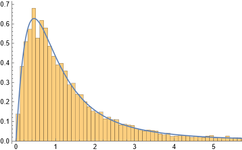
As a partial test of whether this works, take random sample and compare the associated histogram with the density:

n = 10000;
SeedRandom[12345];
rr = randomR[#] & /@ RandomReal[{0, 1}, n];
Show[Histogram[rr, "FreedmanDiaconis", "PDF"],
 Plot[density, {r, 0, 10}]]

Update 1: @kglr in a comment below showed that a random sample can be used with the simpler Mathematica code:

pd = ProbabilityDistribution[density, {r, 0, Infinity}];
SeedRandom[12345];
rr = RandomVariate[pd, n]

Now generate values of $\lambda$. From the relationship given we have:

Solve[ri == (λi - λi1)/(λi1 - λi2), λi][[1, 1, 2]]
(* λi1 + ri λi1 - ri λi2 *)

$$\lambda_i=\lambda_{i-1}+r_i (\lambda_{i-1}- \lambda_{i-2})$$

Putting this all together:

(* Random sample of R values *)
n = 1000;
SeedRandom[12345];
rr = randomR[#] & /@ RandomReal[{0, 1}, n];

(* Generate λ values *)
λλ = ConstantArray[0, n];
λλ[[1]] = 0;
λλ[[2]] = 1;
Do[λλ[[i]] = λλ[[i - 1]] + rr[[i]](λλ[[i - 1]] - λλ[[i - 2]]), {i, 3, n}]

(* Plot results *)
ListPlot[λλ, Frame -> True, FrameLabel -> (Style[#, Italic, 18] &) /@ {"i", "λ[i]"}]

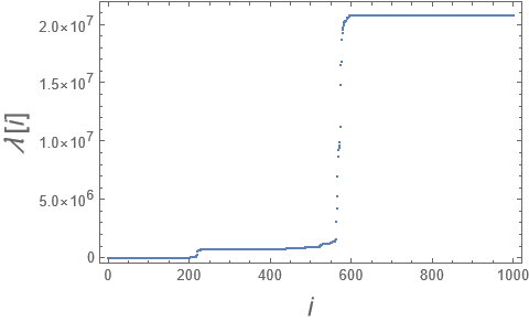
I don't know the subject matter so I have no idea if the resulting figure makes any sense or if the cited paper makes any sense or if I've made an error. All are possible.

Update 2: Finding a nice closed-form formula for the density of $\lambda_i$ does not seem likely as the random variables $\lambda$ become more and more difficult to deal with. We have for the first few $\lambda$ random variables the following pattern:

$$\lambda_3=1+R_3$$ $$\lambda_4=1+R_3+R_3 R_4$$ $$\lambda_5=1+R_3+R_3 R_4+R_3 R_4 R_5$$ $$\lambda_6=1+R_3+R_3 R_4+R_3 R_4 R_5+R_3 R_4 R_5 R_6$$

@kglr also showed how to produce this using the following:

solλ = RSolve[{λ[m] == λ[m - 1] + r[m] (λ[m - 1] - λ[m - 2]), λ[1] == 0, λ[2] == 1},
  λ[m], m][[1]] /. {K[1] -> j, K[2] -> i}

The above can be simplified for each value of $m$:

solλ /. m -> 3 // Expand
(* {λ[3] -> 1 + r[3]} *)

solλ /. m -> 6 // Expand
(* {λ[6] -> 1 + r[3] + r[3] r[4] + r[3] r[4] r[5] + r[3] r[4] r[5] r[6]}

However, one can produce the density for $\lambda_4$ numerically (as opposed to random sampling) by integrating the product of the densities times the Jacobian with r4 replaced by (-1 - r3 + \[Lambda]4)/r3 over r3 ranging from 0 to \[Lambda]4 - 1:

(* Jacobian *)
J = 1/r3;
(* Integrand *)
integrand = FullSimplify[(density /. r -> r3) (density /. r -> (-1 - r3 + λ)/r3) J, 
  Assumptions -> {r3 > 0 && λ > r3 + 1}];
(* Probability density function *)
pdfλ4[λ4_] := NIntegrate[integrand /. λ -> λ4, {r3, 0, λ4 - 1}]

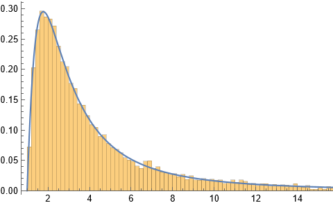
Now to compare with a random sample:

n = 10000;
density = 27 (r + r^2)/(8 (1 + r + r^2)^(5/2));
dist = ProbabilityDistribution[density, {r, 0, ∞}];
SeedRandom[12345];
rr3 = RandomVariate[dist, n];
rr4 = RandomVariate[dist, n];
λλ4 = 1 + rr3 + rr3*rr4;

Show[Histogram[λλ4, "FreedmanDiaconis", "PDF"],
 Plot[pdfλ4[t], {t, 1, 20}]]