Plotting InterpolatingFunction of a solution of Fokker-Planck equation

Question

I want the 3D surface plot of -Log[sol[x,y,8]] but I can't handle the InterpolatingFunction error. Please help me in extracting the function.

delt[x_, y_] := PDF[MultinormalDistribution[{0, 0}, {{.5, 0}, {0, .5}}], {x, 
y}];
b=1; k=1;n=4;S=0.5;a=0.2;
FPE = \!\(\*SubscriptBox[\(\[PartialD]\), \(t\)]\(p[x, y, t]\)\) == s*\!\(\*SubscriptBox[\(\[PartialD]\), \(x, x\)]\(p[x, y, t]\)\) + s*\!\(\*SubscriptBox[\(\[PartialD]\), \(y, y\)]\(p[x, y, t]\)\) - \!\(\*SubscriptBox[\(\[PartialD]\), \(x\)]\((\((\((a*x^n)\)/\((S^n + x^n)\) + \((b*S^n)\)/\((S^n + y^n)\) - k*x)\)*p[x, y, t])\)\) - \!\(\*SubscriptBox[\(\[PartialD]\), \(y\)]\((\((\((\((a*y^n)\)/\((S^n + y^n)\) + \((b*S^n)\)/\((S^n + x^n)\) - k*y)\))\)*p[x, y, t])\)\);
s= .01;
sol = NDSolveValue[ {FPE,p[x, y, 0] == delt[x, y],
p[3, y, t] == 0,
p[0, y, t] == 0,
p[x, 0, t] == 0,
p[x, 3, t] == 0
},p, {t, 0, 10}, {y, 0, 3}, {x, 0, 3}, Method -> {"MethodOfLines", "TemporalVariable" -> t, 
 "SpatialDiscretization" -> {"FiniteElement","MeshOptions"->MaxCellMeasure->0.0005}}];
plot3D[-Log[sol[x,y,8]],{x,0,3},{y,0,3},ColorFunction->"TemperatureMap",PlotRange->All]

Answer 1

Edit2: Added code to back-substitute numerical solution into DE

Edit1: Changed after studying solution

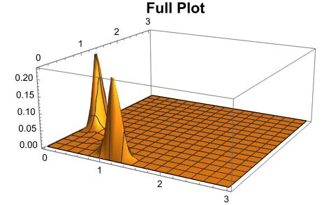
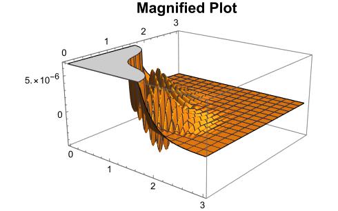
Plotting sol[x,y,8] below one sees it begins very small oscillations between positive and negative values assuming the machine-precision FEM method employed yields and accurate solution and the oscillations aren't spurious. One could back-substitue the solution to check this. Assuming the solution is indeed correct, then this is of course problematic if one is interested in taking the log of the solution unless further processing of the solution is acceptable such as using absolute values or other methods.

Back-substitution of solution into DE:

 (* compute solution with cell measure=0.0005 *)

 cellMeasure = 0.0005;
delt[x_, y_] := 
  PDF[MultinormalDistribution[{0, 0}, {{1/2, 0}, {0, 1/2}}], {x, 
    y}]; 
b = 1; k = 1; n = 4; S = 1/2; a = 2/10;
FPE = \!\(
\*SubscriptBox[\(\[PartialD]\), \(t\)]\(p[x, y, t]\)\) == s*\!\(
\*SubscriptBox[\(\[PartialD]\), \(x, x\)]\(p[x, y, t]\)\) + s*\!\(
\*SubscriptBox[\(\[PartialD]\), \(y, y\)]\(p[x, y, t]\)\) - \!\(
\*SubscriptBox[\(\[PartialD]\), \(x\)]\((\((\((a*x^n)\)/\((S^n + 
            x^n)\) + \((b*S^n)\)/\((S^n + y^n)\) - k*x)\)*
       p[x, y, t])\)\) - \!\(
\*SubscriptBox[\(\[PartialD]\), \(y\)]\((\((\((\((a*y^n)\)/\((S^n + 
             y^n)\) + \((b*S^n)\)/\((S^n + x^n)\) - k*y)\))\)*
       p[x, y, t])\)\);
s = 1/100;
sol = NDSolveValue[ {FPE, p[x, y, 0] == delt[x, y],
    p[3, y, t] == 0,
    p[0, y, t] == 0,
    p[x, 0, t] == 0,
    p[x, 3, t] == 0
    }, p, {t, 0, 10}, {y, 0, 3}, {x, 0, 3}, 
   Method -> {"MethodOfLines", "TemporalVariable" -> t, 
      "SpatialDiscretization" -> {"FiniteElement", 
       "MeshOptions" -> MaxCellMeasure -> cellMeasure}}];

Now plot p(x,y,t) and a yellow trace of p(x,0.8,8) just for visualization:

(* Plot magnified solution and a yellow trace of the solution \
p(x,0.8,8) *)  

trace1 = 
  ParametricPlot3D[{x, 0.8, sol[x, 0.8, 8]}, {x, 0, 3}, 
   PlotStyle -> Yellow, PlotRange -> All];
 magPlot = 
  Plot3D[sol[x, y, 8], {x, 0, 3}, {y, 0, 3}, PlotPoints -> 250, 
   BoxRatios -> {1, 1, 0.5}, 
   PlotLabel -> Style["Magnified Plot", 16, Bold, Black], 
   AxesLabel -> {Style["x", 16, Bold, Black], 
     Style["y", 16, Bold, Black], Style["p(x,y,8)", 16, Bold, Black]},
    ClippingStyle -> None];
Show[{magPlot, trace1}]

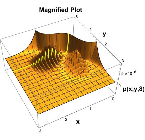
Now compare the left side of the DE with the right side of the DE at the point (1.2,0.8,8) along the yellow trace (or any other point (x,y,8) and print the values:

tVal = 8;
yVal = .8;
xVal = 1.2;
leftSide = (\!\(
\*SubscriptBox[\(\[PartialD]\), \(t\)]\(p[x, y, t]\)\) //. {p -> sol, 
     x -> xVal, y -> yVal, t -> tVal});
rightSide = (s*\!\(
\*SubscriptBox[\(\[PartialD]\), \(x, x\)]\(p[x, y, t]\)\) + s*\!\(
\*SubscriptBox[\(\[PartialD]\), \(y, y\)]\(p[x, y, t]\)\) - \!\(
\*SubscriptBox[\(\[PartialD]\), \(x\)]\((\((\((a*x^n)\)/\((S^n + 
             x^n)\) + \((b*S^n)\)/\((S^n + y^n)\) - k*x)\)*
        p[x, y, t])\)\) - \!\(
\*SubscriptBox[\(\[PartialD]\), \(y\)]\((\((\((\((a*y^n)\)/\((S^n + 
              y^n)\) + \((b*S^n)\)/\((S^n + x^n)\) - k*y)\))\)*
        p[x, y, t])\)\)) //. {p -> sol, x -> xVal, y -> yVal, 
    t -> tVal};

Print["Left side: ", leftSide];
Print["Right side: ", rightSide];

(* Left side: -3.92564*10^-7 *)

(* Right side: 0.0000816017 *)

The difference is not small. I'm not proficient with PDEs and now sure why. You should be able to study this code and test it at other points.