10
$\begingroup$

I have code that generates a Matrix Mat (Mat = data) that, when the graph is plotted, AdjacencyGraph[Mat] gives a graph.

Now, there are many inbuilt functions for GraphLayout. Once we fix a particular GraphLayout. For a particular GraphLayout, we get the vertex coordinates when we use GraphEmbedding.

Let us take a simple example if I have a matrix for a square geometry (square lattice). Then its graph will have a square face. Following the previous paragraph strategy, I will get the coordinates for the vertices like {{0,0}, {0,1},...{0,Lx},...{Ly,Lx}}, where Lx and Ly is the number of vertices along x and y. That is related to the size of the matrix, which is (Lx X Ly) X (Lx X Ly). One can do this for honeycomb or triangle lattices.

However, my graph has higher connectivity that doesn't fall in the above case (meaning it's not Euclidean). Suppose I use the existing GraphLayout. Then the coordinates are not as per the hyperbolic plane. For instance, if I use the GraphLayout -> "SpringElectricalEmbedding" then it uses the particular mechanism (minimizing the spring energy, not important here) to have a graph layout. But it starts to be a problem if I plot different (hyperbolic) graphs, where it is fully messed up and doesn't look good. So I can't extract coordinates rightly.

As an input, I will give the matrix with particular connectivity between the vertices. For example, below, I give as an input a lattice {8,3} in the matrix form, which is a polygon with 8 sides, and at each vertex, three such polygons (octagon) meet. As an output, I want the coordinates for all the vertices so that the coordinates satisfy a hyperbolic distance formula distance[z1,z2]. In other words, it is a fixed distance with a hyperbolic metric. So is there a way to create a custom GraphLayout that does it?

On idea from my side. Maybe we can create an EdgeWeight that encodes the distance function that, in turn, dictates how two edges should be connected? (no idea how good it is, maybe not at all)

MWE:

Mat = data;
graphMat = GraphEmbedding[AdjacencyGraph[ConnectMat, VertexCoordinates -> Coords, VertexLabels -> None, ImageSize -> Large, GraphLayout -> "SpringElectricalEmbedding"]
 distance[z1_, z2_] :=  1./2 ArcCosh[1 + (2 Abs[z1 - z2]^2)/((1 - Abs[z1]^2) (1 - Abs[z2]^2))];

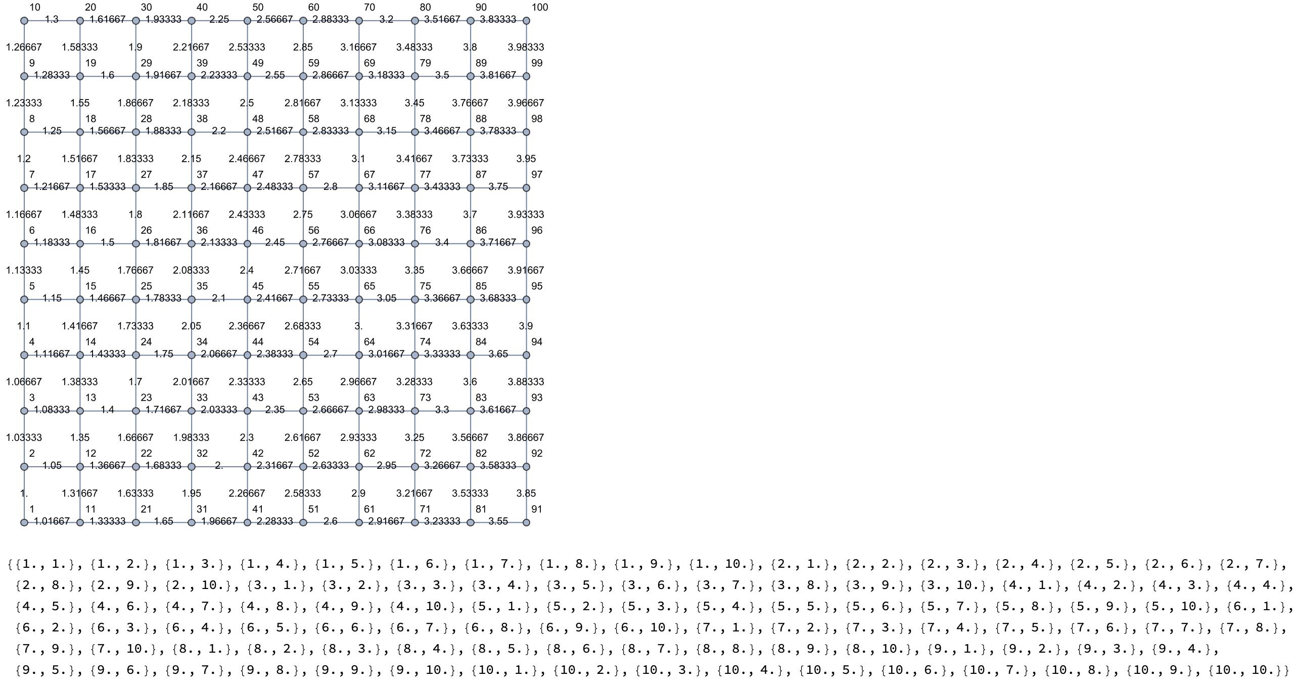
Graph for the above data

Update: Can we use the EdgeWeight function, perhaps? Where this EdgeWeight account for the hyperbolic distance?
One example from Euclidean (not exactly what want though using ChatGPT)

g = GridGraph[{10, 10}, VertexLabels -> "Name", 


EdgeWeight -> Range[1, 4 - 1/60, 1./60], 
   EdgeLabels -> "EdgeWeight"];

distance[v1_, v2_] := Norm[v1 - v2];

calculateLayout[g_, distance_] := 
  Module[{vertices, edges, layout}, vertices = VertexList[g];
   edges = EdgeList[g];
   layout = 
    AssociationThread[vertices, 
     Flatten[Outer[List, Range[10], Range[10]], 1]];
   Do[With[{v1 = First[edge], v2 = Last[edge]}, 
     While[distance[layout[v1], layout[v2]] > 
       PropertyValue[{g, edge}, EdgeWeight], 
      layout[v2] += 0.01*(layout[v1] - layout[v2])]], {edge, edges}];
   layout];

layout = calculateLayout[g, distance];

ambush = 
 Graph[g,(*VertexCoordinates->layout,*)VertexLabels -> "Name"(*,
  EdgeLabels->"EdgeWeight"*)]

GraphEmbedding[ambush]

I would have rather wanted to have the coordinates look like the values on the Edge instead of the original coordinates.

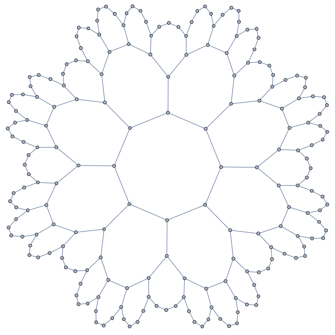
enter image description here

$\endgroup$
14
  • 1
    $\begingroup$ I don't understand the question. From what I can tell you are asking to do multidimensional scaling in hyperbolic space, but it's not clear at all. Please explain better what you want to achieve. What is your input data, what is the specific output you want? $\endgroup$
    – Szabolcs
    Commented May 20, 2023 at 8:14
  • $\begingroup$ @Szabolcs Sorry for getting back late! Sure! Let me paraphrase the statement to make it more clear. Just to say few words to make it little clear to you: I have a Adjacency matrix that has the information of how each nodes (or vertices) are connected to each other. However, this connectivity only exists in hyperbolic space (negatively curved) but if one tries to embed it in Euclidean palne their are distortions (where the edges look smaller if far from origin). $\endgroup$
    – Shamina
    Commented May 22, 2023 at 9:12
  • $\begingroup$ @Szabolcs In order to resovel this problem, I want to get the coordinates for each vertices with a particular metric (Poincaré metric) such that the cooridnates are not of Euclidean type (which will we wrong) by hyperbolic type (that is embedded on a Euclidean plane with the above metric). $\endgroup$
    – Shamina
    Commented May 22, 2023 at 9:12
  • $\begingroup$ @Szabolcs I edited my question to answer your question as clearly as I can. Please have a look :) Let me know if I need to make it clear more. Infinite thanks! $\endgroup$
    – Shamina
    Commented May 22, 2023 at 9:48
  • 1
    $\begingroup$ First, if you want the embedding algorithm to use EdgeWeight, you have to enable it manually. Second, I don't think you can modify the "SpringEmbedding" in any way to account for your metric because you cannot redefine the energy function, and using EdgeWeights will not help because your metric is not translationally invariant. Third, you can try writing your own embedding algorithm – it is in principle just a very simple minimizator (like FindMinimum) with a scoring function being ... $\endgroup$
    – Domen
    Commented May 22, 2023 at 17:35

1 Answer 1

16
$\begingroup$

Not sure if the following is close to what you need, but the pretty pictures it can produce might be of interest.

We define a graph function that takes five arguments and Graph options.

The first argument controls the number of vertices of seed polygon, the second argument controls the rotation/reflections transformations, the third integer specifies the number of iterations, the fourth argument specifies the projection model as Poincare or Beltrami-Klein, the fifth argument controls tolerance used in rationalizing coordinates. The helper functions indexCoords, hCoords, getVertexCoords, getEdgeList and poincareESF are defined in the Code section below.

hyperbolicGraph[n_, m_, iter_ : 1, 
   layout : (Automatic | "Poincare" | "Beltrami") : "Poincare", pr_ : Automatic, 
   opts : OptionsPattern[]] /; (1/n + 1/m < 1/2) := 
 Module[{vl, el, vc,
    coords = indexCoords @ hCoords[n, m, iter, 
      layout, pr /. Automatic -> 10^-5]}, 
  vc = getVertexCoords @ coords; 
  el = getEdgeList @ coords; 
  vl = Range @ Length @ vc;
  Graph[vl, el, VertexCoordinates -> vc,
    EdgeShapeFunction -> poincareESF, opts]] 

Examples

Note: Before using hyperbolicGraph, you need to copy and execute the code in the Code section below.

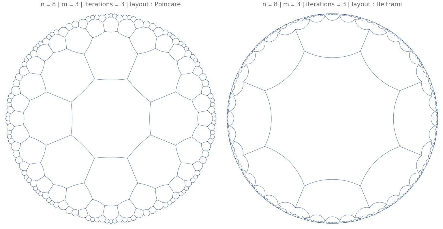
Row[hyperbolicGraph[8, 3, 3, #, Automatic, 
    VertexShapeFunction -> None, 
    PlotLabel -> Style["n = 8 | m = 3 | iterations = 3 | layout : " <> #, 16], 
    ImageSize -> Large] & /@ {"Poincare", "Beltrami"}]

enter image description here

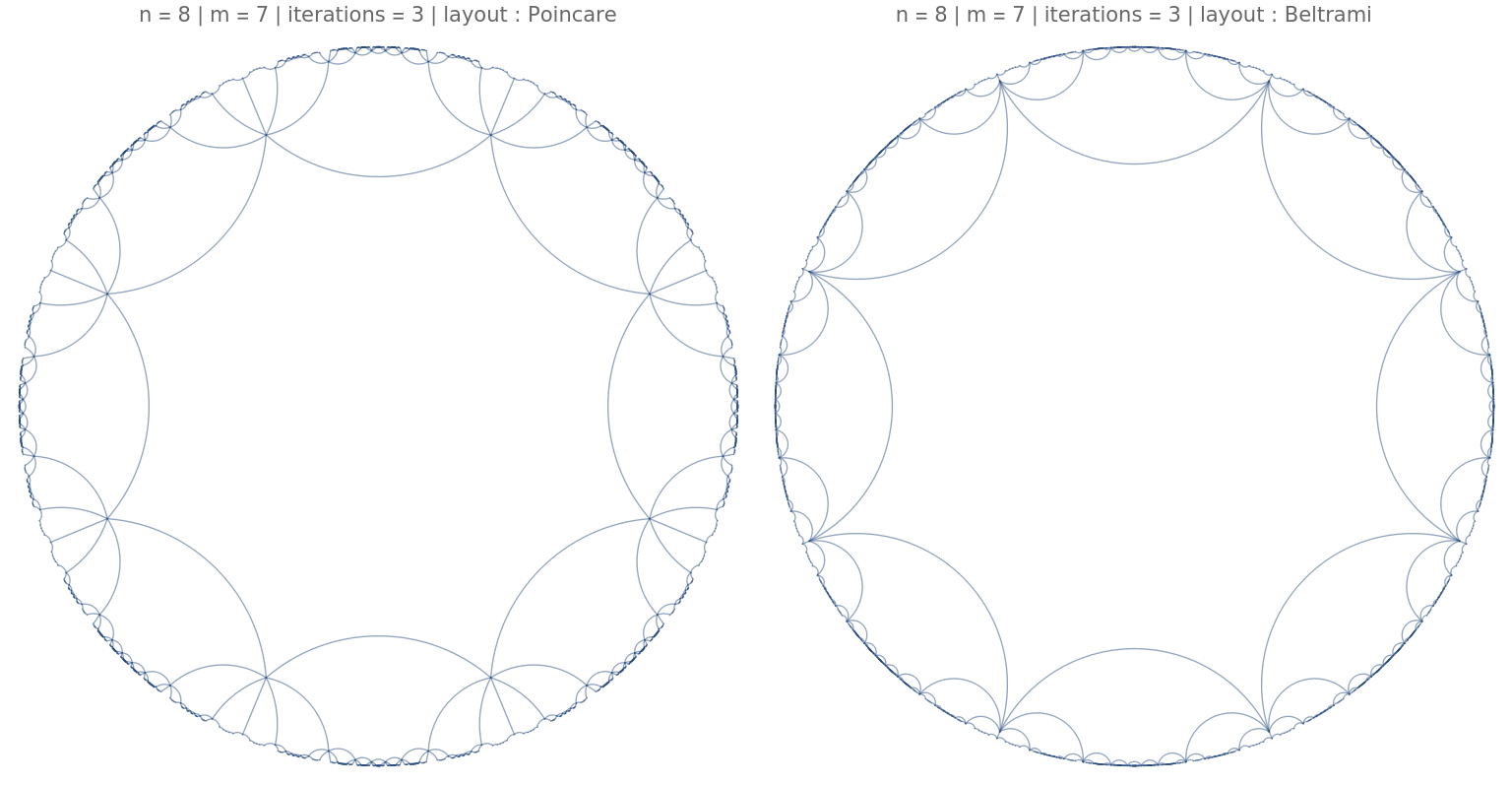
Replace 3 in the second argument with 7 to get:

enter image description here

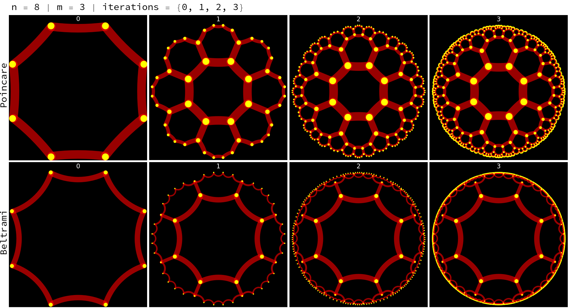
Playing with Graph options for styling edges and vertices:

n = 8; m = 3;

table = Table[With[{ge = GraphEmbedding[#]}, 
  SetProperty[#,
   {EdgeStyle -> {e_ :> Directive[Red, Opacity[.6], 
      AbsoluteThickness[(1.1 - N @ Norm[Mean @ ge[[{e[[1]], e[[-1]]}]]]) 30], 
         CapForm["Round"]]}, 
      VertexStyle -> {v_ :> {Yellow, 
          AbsolutePointSize[(1.1 - N@Norm[ge[[v]]]) 25]}}}]] & @
  hyperbolicGraph[n, m, it, lo, Automatic, 
     PlotLabel -> Style[it, White, 16], 
     VertexShapeFunction -> "Point", GraphStyle -> "ThickEdge", 
     EdgeStyle -> {e_ :> 
        Directive[Opacity[.6], RandomColor[], CapForm["Round"]]}, 
     ImageSize -> 350, Background -> Black], 
 {lo, {"Poincare", "Beltrami"}}, {it, {0, 1, 2, 3}}];

Labeled[Grid[MapThread[Prepend]@
   {table, Style[Rotate[#, 90 Degree], 24] & /@ {"Poincare", "Beltrami"}}],
 Style[StringForm["  n = `` | m = `` | iterations = {0, 1, 2, 3}", n, m], 24], 
 {{Top, Left}}]

enter image description here

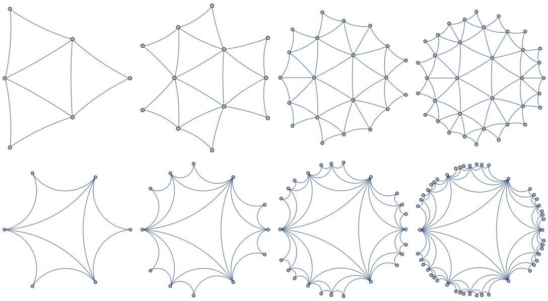
Further examples:

n = 3; layout = Automatic;

Grid[{hyperbolicGraph[n, 7, #, layout, Automatic, 
     ImageSize -> 200] & /@ Range[4], 
  hyperbolicGraph[n, 50, #, layout, Automatic, 
     ImageSize -> 200] & /@ Range[4]}]

enter image description here

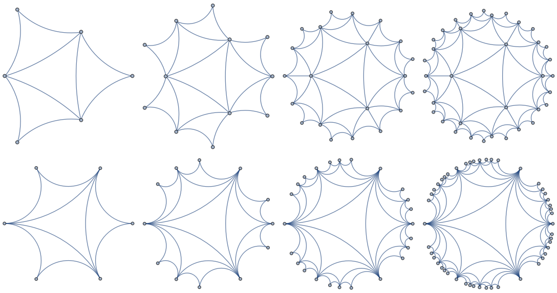
With layout = "Beltrami" we get

enter image description here

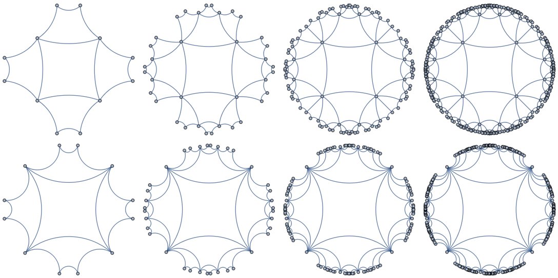
With n = 4; layout = Automatic; we get

enter image description here

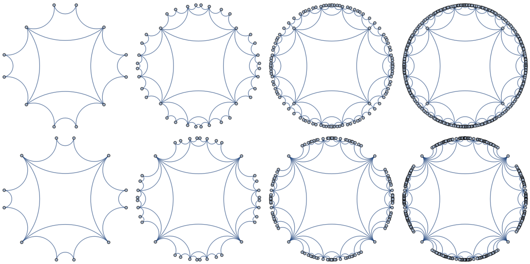
With n = 4; layout = "Beltrami"; we get

enter image description here

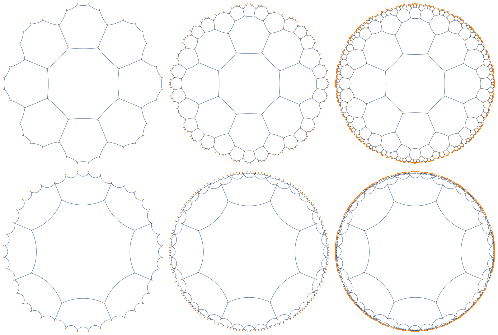
Column[Table[
  Row[hyperbolicGraph[8, 3, #, layout, Automatic, ImageSize -> 400, 
     VertexShapeFunction -> "Point", 
     VertexStyle -> Directive[Orange, PointSize[Small]]] & /@ {1, 2, 3}],
  {layout, {Automatic, "Beltrami"}}]]

enter image description here


Code

First, several functions for generation and transformations of lists of coordinates (these are slightly modified versions of functions I found inspecting the function GraphComputation`RegularHyperbolicTilingGraphGraphComputation`RegularHyperbolicTilingGraph):

ClearAll[hyperbolicRotation, hyperbolicReflection, growCoords,  seedCoords,
  hCoords, hyperbolicGraph]

hyperbolicRotation[z_, {c_, t_}] := 
 With[{w = ((z - c) E^(I t))/(1 - z Conjugate[c])},
   (c + w)/(1 +  w Conjugate[c])] 

hyperbolicReflection[coords_, n_, m_] /; (1/n + 1/m < 1/2) := 
 Nest[Append[#, hyperbolicRotation[#[[-2]], {#[[-1]], 2 π/m}]] &, coords, n - 2]

seedCoords[n_, m_] /; (1/n + 1/m < 1/2) := 
 Block[{r, v, s = Sin[π/n]^2  Sec[π/m]^2}, r = s/(1 - s); 
  v = Sqrt[1 + 2 r - 2 Sqrt[r (1 + r)] Sin[π (1/n + 1/m)]] Exp[I π/n ]; 
  NestList[hyperbolicRotation[#, {0, -2 π/n }] &, v, n - 1]]

growCoords[coords_, m_] := With[{n = Length[coords]}, 
  Map[hyperbolicReflection[#, n, m] &] @ Reverse[Partition[coords, 2, 1, 1], 2]]

We use the above functions to generate a nested list of coordinates:

hCoords[n_, m_, k_, op : (Automatic | "Poincare" | "Beltrami") : "Poincare", 
   pr_ : Automatic ] /; (1/n + 1/m < 1/2) := 
 Module[{opr = op /. 
   {Automatic | "Poincare" ->  Identity, 
   "Beltrami" -> (2 #/(1 + Abs[#]^2) &)}}, 
  Rationalize[Map[ReIm @* opr, 
    NestList[p |-> Flatten[growCoords[#, m] & /@ p, 1],
    {N @ seedCoords[n, m]}, k], {2}], pr /. Automatic -> 10^-5]]

Next, a few operators to get the edge list, vertex list and vertex coordinates from the coordinate list produced by hCoords:

indexCoords = Association @* DeleteDuplicatesBy[Sort @* First] @* 
  (Thread[ArrayComponents[#, 2] -> #] &) @* Last;

getEdgeList = DeleteDuplicatesBy[Sort] @* Apply[Join] @*
   Map[MapApply[UndirectedEdge]@Partition[#, 2, 1, 1] &] @* Keys;

getVertexCoords = DeleteDuplicates @* Apply[Join] @* KeyValueMap[Thread[#->#2]&];

For hyperbolic lines and segments we use the function GraphComputation`GraphChartDump`geo

GraphComputation`GraphPropertyChart;

poincareESF = GraphComputation`GraphChartDump`geo[.99 First[#], .99 Last[#], 
    "segment"] &;

poincareLine = GraphComputation`GraphChartDump`geo[.99 First[#], .99 Last[#], 
    "line"] &;

We now have all the pieces to define hyperbolicGraph:

hyperbolicGraph[n_, m_, iter_ : 1, 
   layout : (Automatic | "Poincare" | "Beltrami") : "Poincare", pr_ : Automatic, 
   opts : OptionsPattern[]] /; (1/n + 1/m < 1/2) := 
 Module[{vl, el, vc,
    coords = indexCoords @ hCoords[n, m, iter, 
      layout, pr /. Automatic -> 10^-5]}, 
  vc = getVertexCoords @ coords; 
  el = getEdgeList @ coords; 
  vl = Range @ Length @ vc;
  Graph[vl, el, VertexCoordinates -> vc,
    EdgeShapeFunction -> poincareESF, opts]] 

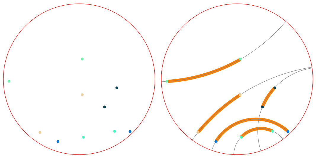
Poincare lines and segments

SeedRandom[12];
rp = RandomPoint[Disk[], {5, 2}];
colors = RandomColor[5];

Row[{Graphics[{Red, Circle[], Blue, PointSize[Large], 
    MapThread[{#, Point@#2} &]@{colors, rp}}, ImageSize -> 400],
  Graphics[{Red, Circle[], CapForm["Butt"], AbsoluteThickness[8], 
    Orange, poincareESF /@ rp, Gray, AbsoluteThickness[1], 
    poincareLine /@ rp, Blue, PointSize[Large], 
    MapThread[{#, Point@#2} &]@{colors, rp}}, ImageSize -> 400]}]

enter image description here


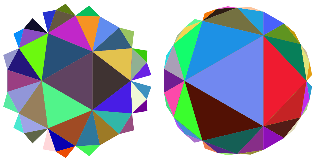
Fun with hCoords:

n = 3; m = 8;

Row[Graphics[{RandomColor[], Polygon @ #} & /@ 
   Flatten[hCoords[n, m, 4, #], 1], ImageSize -> 400] & /@ 
    {"Poincare", "Beltrami"}, Spacer[10]]

enter image description here

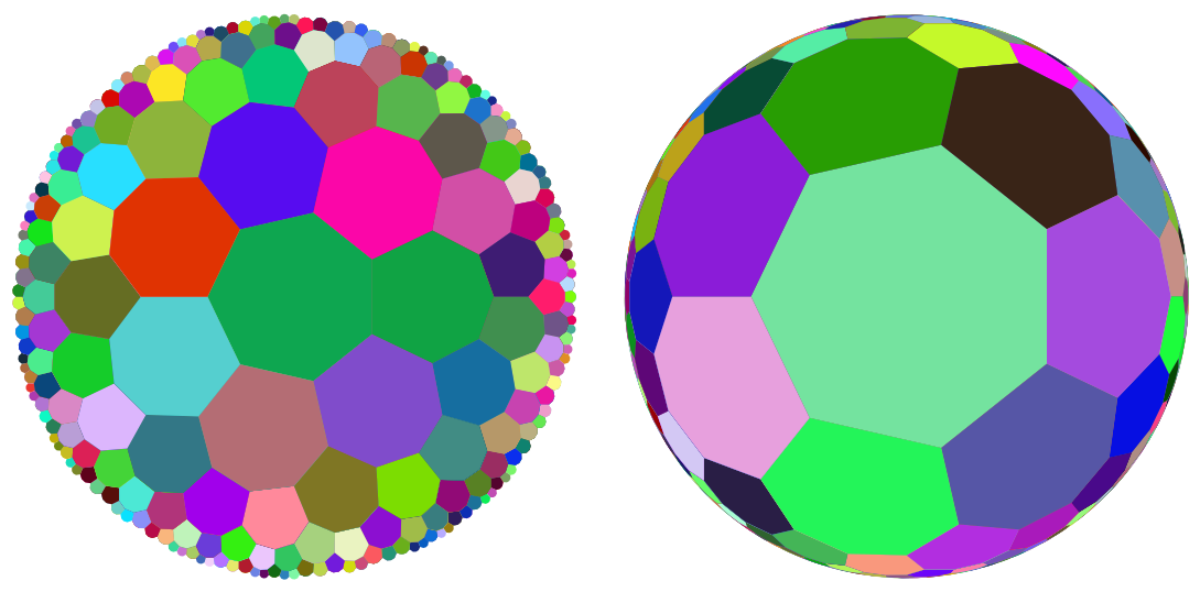
With n = 7; m = 3; we get

enter image description here

$\endgroup$
7
  • $\begingroup$ Great answer! Can we get the adjacency matrix at a fixed iteration(e.g., it=2) from these results? $\endgroup$
    – Shasa
    Commented Jun 1, 2023 at 8:04
  • 1
    $\begingroup$ use AdjacencyMatrix @ hyperbolicGraph[3, 7, 2]? $\endgroup$
    – kglr
    Commented Jun 1, 2023 at 9:00
  • $\begingroup$ Great! Thank you very much! $\endgroup$
    – Shasa
    Commented Jun 1, 2023 at 9:34
  • $\begingroup$ Thank you so much for your answer @kglr! Sorry for the late response. I thought no will answer it. Here is your beautiful answer! I tried to run your code but I think I'm making some mistakes. I'm getting errors instead of beautiful plots. $\endgroup$
    – Shamina
    Commented Jun 5, 2023 at 11:58
  • 2
    $\begingroup$ use GraphEmbedding@hyperbolicGraph[8, 3, 2] ? $\endgroup$
    – kglr
    Commented Jun 5, 2023 at 13:20

Your Answer

By clicking “Post Your Answer”, you agree to our terms of service and acknowledge you have read our privacy policy.

Not the answer you're looking for? Browse other questions tagged or ask your own question.