Implementing a way of generating binary data for use in a logistic regression

Question

Background

I want to generate a set of test data to be used in a logisitic regression.

As an example consider the scenario where a cannonball is fired at a wall. There are only two outcomes: the wall collapses (1) and the wall does not collapse (0). I'm interested in the probability that the wall collapses as a function of the cannonball velocity. It is reasonable to expect that the probability vs velocity will have an S shape. Nevertheless, it is just an example.

I want to implement a procedure of generating datapoints according to the so--called K-in-a-row method. The dataset generated by this method is said to be useful in determining the velocity $V_{10}$ where the cannonball has a 10% chance of breaking the wall.

The K-in-a-row procedure works like this

1. Choose some starting velocity
2. If the wall collapses (y_i=1) for a particular velocity, decrease the velocity by a fixed amount
3. If the wall does not collapse (y_i=0) k times in a row for a particular velocity, increase the velocity by a fixed amount

I'm interested in generating data on the form $\{V_i,y_i\}$ where $V_i$ is the velocity and $y_i=\{0,1\}$ describes whether the wall collapses or not.

As an example I consider the "true" distribution to be $$P(y_i=1|x_i)=\frac{1}{1+e^{-\frac{x-\mu}{s}}}$$ where the mean is $\mu = 50$ and the scale is $s=13$. I then pick $0$ or $1$ from a Bernoulli distribution with a probability given by the expression above.

Implemented code

The concrete code for generating the data is given below.

(*Parameter of "True distribution" and step velocity step size*)
s = 13; \[Mu] = 50; 
step = 5;
(*Generate data according to K-in-a-row test*)
dataKinRow = {};
k = 5;
(*First shot*)
V0 = 20;
collapse = RandomVariate[
    BernoulliDistribution[1/(1 + E^(-((V0 - \[Mu])/s)))], 1][[1]];


Table[
  
  If[
   collapse == 1,
   
   AppendTo[dataKinRow, {V0, collapse}]; 
   V0 = V0 - step;
   collapse = 
    RandomVariate[
      BernoulliDistribution[1/(1 + E^(-((V0 - \[Mu])/s)))], 1][[1]];
   ,
   
   n = 1;
   While[
    collapse == 0 && n <= k,
    AppendTo[dataKinRow, {V0, collapse}];
    collapse = 
     RandomVariate[
       BernoulliDistribution[1/(1 + E^(-((V0 - \[Mu])/s)))], 1][[1]];
    n = n + 1;
    ];
   
   Which[
    collapse == 1 && n == 6, V0 = V0 - step,
    collapse == 1 && n != 6, AppendTo[dataKinRow, {V0, collapse}]; 
    V0 = V0 - step,
    collapse == 0, V0 = V0 + step
    ]
   
   ]
  
  , {shotNumber, 1, 500}];
(*Generate data according to K-in-a-row test*)
dataKinRow = {};
k = 5;
(*First shot*)
V0 = 20;
collapse = RandomVariate[
    BernoulliDistribution[1/(1 + E^(-((V0 - \[Mu])/s)))], 1][[1]];


Table[
  
  If[
   collapse == 1,
   
   AppendTo[dataKinRow, {V0, collapse}]; 
   V0 = V0 - step;
   collapse= 
    RandomVariate[
      BernoulliDistribution[1/(1 + E^(-((V0 - \[Mu])/s)))], 1][[1]];
   ,
   
   n = 1;
   While[
    collapse== 0 && n <= k,
    AppendTo[dataKinRow, {V0, collapse}];
    collapse= 
     RandomVariate[
       BernoulliDistribution[1/(1 + E^(-((V0 - \[Mu])/s)))], 1][[1]];
    n = n + 1;
    ];
   
   Which[
    collapse== 1 && n == 6, V0 = V0 - step,
    collapse== 1 && n != 6, AppendTo[dataKinRow, {V0, collapse}]; 
    V0 = V0 - step,
    collapse== 0, V0 = V0 + step
    ]
   
   ]
  
  , {shotNumber, 1, 500}];

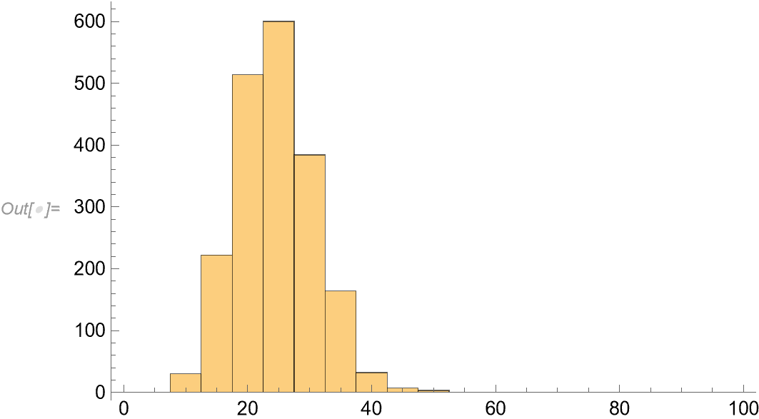
The output for the dataset seems reasonable, although I am a bit unsure if my while-loop and what happens directly after it is correct.

I can then perform a logistic distribution to my set of data with prediction intervals on the probability by doing the following:

(*Fit logistic regression model*)
lmfKinROW = LogitModelFit[dataKinRow, x, x];
Normal[lmfKinROW]

(*Get estimated parameters and associated covariance matrix*)
parmsKinROW = lmfKinROW["BestFitParameters"];
lmfKinROW["ParameterTable"]
N[{\[Mu]/s, -1/s}]
covKinRow = lmfKinROW["CovarianceMatrix"]

Show[
 Plot[1/(1 + E^(-((x - \[Mu])/s))), {x, \[Mu] - 5*s, \[Mu] + 5*s}, 
  PlotStyle -> Thick, PlotRange -> {All, {-0.1, 1.1}}],
 ListPlot[dataKinRow],
 Plot[
  {0.1,
   1 - (1/(1 + Exp[parmsKinROW . {1, x}])),
   1 - 1/(1 + 
       Exp[parmsKinROW . {1, x} - 
         1.96 Sqrt[{1, x} . covKinRow . {1, x}]]),
   1 - 1/(1 + 
       Exp[parmsKinROW . {1, x} + 
         1.96 Sqrt[{1, x} . covKinRow . {1, x}]]),
   }, {x, \[Mu] - 5*s, \[Mu] + 5*s}, PlotRange -> {All, {-0.1, 1.1}}, 
  Frame -> True, 
  PlotStyle -> {Red, Red, {Black, Dotted}, {Black, Dotted}}]]

Question & issue

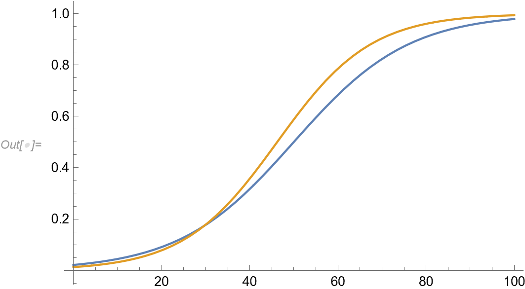
To my great dissatisfaction I find that the logistic distribution does not seem to converge to the "true" distribution despite if I include a large number of cannonball shots. The true distribution even lies outside of the confidence intervals. Furthermore, the logistic regression for k-in-a-row converges worse than the regression i obtain just picking velocities from a uniform distribution and use the Bernoulli distribution in the same way as above to determine collapse/not collapse. This might be because the method generates data that are focused towards smaller velocities, but I would at least expect the estimate for $V_{10}$ to be better.

Unfortunately, my question then reduces to something I hope is not too trivial for this site: is there anything wrong with the way I generate my set of data, specifically with the implemented k-in-a-row algorithm?

Answer 1

I think that the data generation matches your description (although it could be done more compactly) and while I'm not crazy about all of the lack of independence among the samples, the maximum likelihood approach of LogitModelFit gets you appropriate estimates of the parameters. (I think the measures of precision must be a bit suspect because of the lack of independence among the samples but that's another issue.)

Your settings of the initial velocity, step size, and value of $k$ (and maybe the whole approach) doesn't seem to get a wide range of values of the predictor variable making it difficult to get a good estimate of the underlying function.

So your "dissatisfaction" is simply that your data generation approach just doesn't work very well to meet your expectations. That has nothing to do with LogisticModelFit.

Here is a more compact approach to generating that kind of data:

(* Function to generate samples and next velocity *)
f[v_, μ_, s_, k_, Δ_] := Module[{p, probs, x},
  p = 1/(1 + Exp[-(v - μ)/s]);
  probs = Table[If[i == k, (1 - p)^k, p (1 - p)^i], {i, 0, k}];
  x = RandomChoice[probs -> Range[0, k]];
  If[x == k, {v + Δ, Table[{v, 0}, {i, k}]},
   If[x == 0, {v - Δ, {{v, 1}}}, {v - Δ, 
     Join[{{v, 1}}, Table[{v, 0}, {i, x}]]}]]
  ]

(* Set values of parameters *)
{v0, μ, s, k, Δ} = {20, 50, 13, 5, 5};

(* Generate samples *)
n = 500;  (* Sample size *)
SeedRandom[12345];
data = {};  (* Initialize data *)
Do[y = f[v0, μ, s, k, Δ];
 v0 = y[[1]];  (* Get updated velocity *)
 data = Join[data, y[[2]]],  (* Append new data *)
 {j, n}]

Now perform the analysis:

(* Logistic regression *)
lmf = LogitModelFit[data, x, x];

(* Solve for the estimates of s and μ *)
sol = Solve[{-mu/ss, 1/ss} == lmf["BestFitParameters"], {mu, ss}]
(* {mu -> 46.2388, ss -> 10.5968} *)

(* Plot true and fitted curve *)
Plot[{1/(1 + Exp[-(v - μ)/s]), 
  1/(1 + Exp[-(v - mu)/ss] /. sol)}, {v, 0, 100}]

(* Histogram of predictor variables *)
Histogram[data[[All, 1]], "FreedmanDiaconis", 
 PlotRange -> {{0, 100}, Automatic}]

The upper values of the predictor just aren't very well represented.