TL;DR
listA = {0.3, 0.6, 0.6, 0.9}
listB = {0.1, 0.2, 0.3, 0.4}
threshold = 10^-15;
(*Revised and better way thanks to J.M.*)
f[list1_, list2_, Method -> "Unitize"] := (1 - Unitize[Chop[Outer[Plus, list1, -list1], threshold]]).list2
(*Old*)
f[list1_, list2_, Method -> "Boole"] := Outer[Boole[Chop[#1 - #2, threshold] == 0] &, list1, list1].list2
(*Run-Length Block Diagonal Matrix*)
f[list1_, list2_, Method -> "RLBDM"] := Block[
{runs, runLengthMatrixList},
runs = Split[list1, Abs[#1 - #2] < 10^-15 &];
runLengthMatrixList = ConstantArray[1, Length@# {1, 1}] & /@ runs;
(*see below*) matrixDirectSum[runLengthMatrixList].list2
]
(*SequencePosition*)
f[list1_, list2_, Method -> "SequencePosition"] := Block[
{temp = list2, pos = SplitBy[SequencePosition[list1, {x_, (x_) ..}], #[[2]] &][[;; , 1]]},
(temp[[Span @@ #]] = Total@Take[list2, #]) & /@ pos;
temp
]
f[listA, listB, Method -> #] & /@ {"Boole", "Unitize", "RLBDM", "SequencePosition"}
{{0.1, 0.5, 0.5, 0.4}, {0.1, 0.5, 0.5, 0.4}, {0.1, 0.5, 0.5, 0.4}, {0.1, 0.5, 0.5, 0.4}}
The Long Part
WE CaN seE that $\left(
\begin{array}{cccc}
1 & 0 & 0 & 0 \\
0 & 1 & 1 & 0 \\
0 & 1 & 1 & 0 \\
0 & 0 & 0 & 1 \\
\end{array}
\right) \cdot \left(
\begin{array}{c}
w \\
x \\
y \\
z \\
\end{array}
\right) = \left(
\begin{array}{c}
w \\
x + y \\
x + y \\
z \\
\end{array}
\right)$ where the block-, sub-matrix of 1s comes from the positions (or position and length of the run since they will always be adjacent) of the duplicate elements. Now it's just a matter of creating that matrix from the secondary vector.
Outer Product
One way of going about making the transformation is using the outer product Outer to element-wise identify the entries that are within the threshold of each other.
f[list1_, list2_, Method -> "Boole"] := Outer[Boole[Chop[#1 - #2, 10^-15] == 0] &, list1, list1].list2
f[list1_, list2_, Method -> "Unitize"] :=  (*Thanks J.M.*) (1 - Unitize[Chop[Outer[Plus, list1, -list1], 10^-15]]).list2
Matrix Direct Sum and Run-Length Block Diagonal Matrix
Another method is to take advantage of the fact that the duplicate elements will always be adjacent, thus creating runs of identical entries. The length of these runs (including runs of length 1) is exactly the dimension of the block matrix that appears on the diagonal of our transformation. Then we can compute the direct sum of these matrices (i.e. a block diagonal matrix whose diagonal entries are the run-matrices).
matrixDirectSum[matList : {__?MatrixQ}] := SparseArray`SparseBlockMatrix[Transpose@Range[1, Length@matList {1, 1}] -> matList // Thread] // Normal

f[list1_, list2_, Method -> "RLBDM"] := Block[
  {runs, runLengthMatrixList},
  runs = Split[list1, Abs[#1 - #2] < 10^-15 &] (*Partition the list into runs of entries that are within the threshold*);
  runLengthMatrixList = ConstantArray[1, Length@# {1, 1}] & /@ runs (*Create a list of square 1-matrices with dimension equal to the length of the run*);
  matrixDirectSum[runLengthMatrixList].list2
]
SparseArray`SparseBlockMatrix found via tumbling down the rabbit hole of this question to this question and finally to this question. I have also had this nagging feeling that the block matrix could be constructed more directly via Kronecker sums and/or Kronecker products.
SequencePosition
In doing something else, using SequencePosition also popped into my head.
f[list1_, list2_, Method -> "SequencePosition"] := Block[
  {temp = list2, pos = SplitBy[SequencePosition[list1, {x_, (x_) ..}], #[[2]] &][[;; , 1]]},
  (temp[[Span @@ #]] = Total@Take[list2, #]) & /@ pos;
  temp
]
This even works as below because it takes and adds the orthogonal rows of the identity matrix.
Just the matrix
In any case, we can also implement the functionality to give just the matrix.
f[list_, m : (Method -> _)] := f[list, IdentityMatrix@Length@list, m]
f[listA, Method -> "RLBDM"]
$\left(
\begin{array}{cccc}
1 & 0 & 0 & 0 \\
0 & 1 & 1 & 0 \\
0 & 1 & 1 & 0 \\
0 & 0 & 0 & 1 \\
\end{array}
\right)$
This is also the form of an adjacency matrix of the graph representation of the matrix.
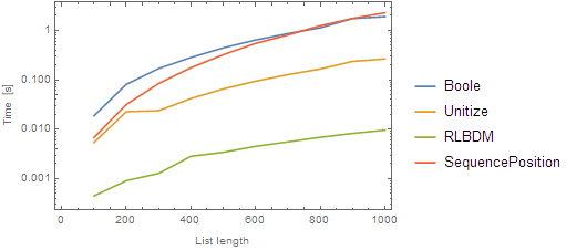
Timing Comparison
With[
  {lists = Round[RandomReal[1, {2, #}], 0.1]},
    First@RepeatedTiming[
      f[## & @@ lists, Method -> #];] & /@ {"Boole", "Unitize", "RLBDM", "SequencePosition"}
] & /@ Range[100, 1000, 100] // Transpose
ListLogPlot[
  %,
  DataRange -> {100, 1000},
  PlotLegends -> {"Boole", "Unitize", "RLBDM", "SequencePosition"},
  Joined -> True, Axes -> False, Frame -> True,
  FrameLabel -> {"List length", "Time [s]"}
] // Rasterize
Turns out the RLBDM method is at least an order of magnitude quicker than the others! And as expected, SequencePosition is slowest at higher lengths, no doubt due to pattern matching.


listAis sorted from least to greatest, so they are always adjacent $\endgroup$