3
$\begingroup$

I need to plot massive data stored in external ASCII files. Below is the Mathematica code I use for this job:

Clear["Global`*"];

SetDirectory[" ... "];

dataRG = ReadList["dataRG.out", Number, RecordLists -> True];
dataCH = ReadList["dataCH.out", Number, RecordLists -> True];

Vd = -((Md*(1 + δ))/
Sqrt[(1 + δ)*(b^2 + y^2) + 
x^2 + (a + Sqrt[h^2 + (1 + δ^2)*z^2])^2]);
Vn = -(Mn/Sqrt[x^2 + y^2 + z^2 + cn^2]);
Vh = -(Mh/Sqrt[x^2 + y^2 + z^2 + ch^2]);
V = Vd + Vn + Vh;

Md = 8200; b = 8; a = 3; h = 0.3; δ = 0.1;
Mn = 400; cn = 0.25;
Mh = 0; ch = 25;
E0 = -700;
z0 = 1;

f[x_, px_] := 1/2*px^2 + V /. {y -> 0, z -> z0};

xmax = 11;
pxmax = 41;
plrange = {{-xmax, xmax}, {-pxmax, pxmax}};

C0 = ContourPlot[Evaluate[f[x, px]], {x, -20, 20}, {px, -80, 80}, 
Contours -> {E0}, ContourStyle -> {Black, Thick}, AspectRatio -> 1,
ContourShading -> False, PlotPoints -> 200, 
PerformanceGoal -> "Speed", PlotRange -> plrange];

S1 = ListPlot[Flatten[List /@ dataRG[[All, {1, 2}]], 1], 
PlotStyle -> {GrayLevel[0.8], PointSize[0.003]}];
S2 = ListPlot[Flatten[List /@ dataCH[[All, {1, 2}]], 1], 
PlotStyle -> {GrayLevel[0.05], PointSize[0.003]}];
P0 = Show[{S1, S2, C0}, Frame -> True, Axes -> False, 
FrameLabel -> {"x", OverDot["x"]}, RotateLabel -> False, 
FrameStyle -> Directive[FontSize -> 17, FontFamily -> "Helvetica"], 
AspectRatio -> 1, PlotRange -> plrange, ImageSize -> 550]

which produces the following output

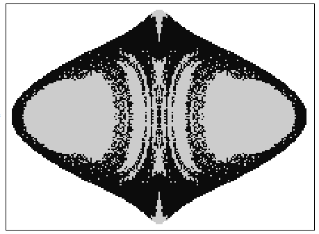
my plot

As you may see from the image two are the main issues:

(1). How can I get rid off the vertical blank gaps?
(2). Why there are some "bold horizontal lines" in the plot and again how can I get rid off them?

I observed, that both issues are influenced by the ImageSize option. In particular, if you play with this option between 400 and 600, it might eliminate the problems. However, I suspect that the cause must be something more profound. So, I would be very grateful, if you suggest me how can I solve these issues and also if you could provide me with a more correct way to plot my data files.

Many many thanks in advance!

Both data files can be found here: dataRG and dataCH.

$\endgroup$
3
  • 1
    $\begingroup$ Quite likely, those things you're seeing are moiré artifacts... $\endgroup$ Commented Jun 10, 2013 at 17:30
  • $\begingroup$ @0x4A4D They could be artifacts, but when I export the plot in different formats (.eps, .pdf, .jpg) they are still present messing up with my plot. $\endgroup$
    – Vaggelis_Z
    Commented Jun 10, 2013 at 17:59
  • $\begingroup$ Though I didn't check your data, I agree with 0x4A4D it might be moiré pattern. One way is to blur them a little when the distance between your adjacent points comes near the DPI of your monitor. $\endgroup$
    – Silvia
    Commented Jun 10, 2013 at 18:24

4 Answers 4

6
$\begingroup$

Your data is on a regular grid, so it is also possible to put each data point into a matrix element, then use functions like ArrayPlot/MatrixPlot to efficiently plot it.

posCH = Reverse[{100, 73} + #/{1, 5}] & /@
                Union[Round[10 dataCH[[All, 1 ;; 2]]]];

posRG = Reverse[{100, 73} + #/{1, 5}] & /@
                Union[Round[10 dataRG[[All, 1 ;; 2]]]];

S12Array = SparseArray[{
                 posRG -> ConstantArray[.8, Length@posRG],
                 posCH -> ConstantArray[.05, Length@posCH]
                 }, {145, 200}, 1];

S12 = ArrayPlot[S12Array, ColorFunction -> GrayLevel, ColorFunctionScaling -> False]

S1 and S2

In order to match C0 (of which I changed the color to Red for highlighting) on it, we need to transform C0:

C0trans = C0 /. {
      GraphicsComplex[pts_, others__] :>
                     GraphicsComplex[{100, 73} + 10 #/{1, 5} & /@ pts, others],
      (PlotRange -> _) :>
                    (PlotRange -> ({100, 73} + 10 #/{1, 5} & /@
                                  (plrange\[Transpose])\[Transpose]))}

And we'll have to construct the FrameTicks manually:

xticks = Join[
   {100 + 10 #, #, {.01, 0}} & /@ Range[-20, 20, 2],
   {100 + 10 #, "", {.005, 0}} & /@ Range[-20, 20, 1/4]];
xticks2 = Join[
   {100 + 10 #, "", {.01, 0}} & /@ Range[-20, 20, 2],
   {100 + 10 #, "", {.005, 0}} & /@ Range[-20, 20, 1/4]];
yticks = Join[
   {73 + (10 #)/5, #, {.01, 0}} & /@ Range[-80, 80, 5],
   {73 + (10 #)/5, "", {.005, 0}} & /@ Range[-80, 80, 1]];
yticks2 = Join[
   {73 + (10 #)/5, "", {.01, 0}} & /@ Range[-80, 80, 5],
   {73 + (10 #)/5, "", {.005, 0}} & /@ Range[-80, 80, 1]];

Combine them:

Show[S12, C0trans,
 FrameTicks -> {{yticks, yticks2}, {xticks, xticks2}},
 FrameLabel -> {"x", OverDot["x"]}, RotateLabel -> False,
 FrameStyle -> Directive[FontSize -> 17, FontFamily -> "Helvetica"],
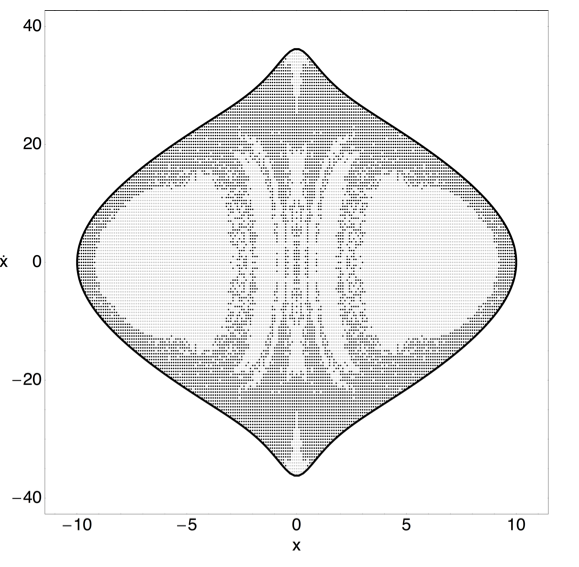
 AspectRatio -> 1, ImageSize -> 550]

combined graph

$\endgroup$
2
  • $\begingroup$ Also try the ArrayPlot with setting the PixelConstrained -> True option. $\endgroup$
    – shrx
    Commented Jun 14, 2013 at 19:18
  • $\begingroup$ @shrx Thanks. This option does make the plot prettier. I didn't adopt it because OP explicitly specified ImageSize -> 550, which will contradict the PixelConstrained -> True or PixelConstrained -> 1 option. $\endgroup$
    – Silvia
    Commented Jun 15, 2013 at 7:12
4
$\begingroup$

You are forcing a regular pattern (your data) on a regular grid with a different spacing. This is bound to lead to aliasing. In your data vertical steps are 5 times larger than the horizontal steps:

Differences@(dataRG[[All, 1]] // Union) // Union

{0.1, 0.1, 0.1, 0.1, 0.1, 0.1, 0.1, 0.1}

Differences@(dataRG[[All, 2]] // Union) // Union

{0.5, 1., 2.5}

The AspectRatio->1 setting forces the data range ratio of ...

 ((Subtract @@ #2)/)Subtract @@ #1)) & @@ (P0 // PlotRange)

3.7272727273.72

to be 1, making the vertical step size a non-integer multiple of the horizontal one. That's trouble.

You will note that if you set AspectRatio->Automatic and the graphics size is sufficient the aliasing is gone.

$\endgroup$
2
  • $\begingroup$ If I set AspectRatio->Automatic the plot is too elongated at the vertical axes and therefore distorted! I want to believe that there is a much simpler solution which we haven't thought yet. $\endgroup$
    – Vaggelis_Z
    Commented Jun 10, 2013 at 21:01
  • $\begingroup$ @Vaggelis_Z As Sylvia already mentioned you could blur your data. $\endgroup$ Commented Jun 10, 2013 at 21:17
4
$\begingroup$

Another possible way would be to use Interpolation (Caution: Very slow!):

posRG = Union[dataRG[[All, {1, 2}]]];

posCH = Union[dataCH[[All, {1, 2}]]];

posBoundary = Cases[C0, GraphicsComplex[pts_, __] :> pts, ∞][[1, 
   Most[Cases[C0, Line[pts__] :> pts, ∞][[1]]]]];

interpFunc = Interpolation[
                  Join[{#, .8} & /@ posRG,
                       {#, .05} & /@ posCH,
                       {#, .05} & /@ posBoundary]]

S12 = DensityPlot[interpFunc[x, y], {x, -10, 10}, {y, -40, 40},
            PlotRange -> {0, 1}, PlotPoints -> 100,
            ColorFunction -> GrayLevel, ColorFunctionScaling -> False,
            RegionFunction -> Function[{x, y, z}, Evaluate[f[x, px] < E0 /. px -> y]]]

P0 = Show[{S12, C0}, Frame -> True, Axes -> False, 
          FrameLabel -> {"x", OverDot["x"]}, RotateLabel -> False, 
          FrameStyle -> Directive[FontSize -> 17, FontFamily -> "Helvetica"], 
          AspectRatio -> 1, PlotRange -> plrange, ImageSize -> 550]

enter image description here

$\endgroup$
4
$\begingroup$

You could render it as a bitmap at a higher resolution, then scale it back down to size. The image scaling algorithms will do a better job of representing the fine detail than ListPlot. This can be done easily with Rasterize. For example, you can do

Rasterize[
 Show[{S1, S2, C0}, Frame -> True, Axes -> False, 
  FrameLabel -> {"x", OverDot["x"]}, RotateLabel -> False, 
  FrameStyle -> Directive[FontSize -> 17, FontFamily -> "Helvetica"], 
  AspectRatio -> 1, PlotRange -> plrange, ImageSize -> 550], 
 RasterSize -> 550*8]

Rasterized version of plot

Note that the resulting object is a bitmap, so won't look good if you try to resize it.

$\endgroup$

Your Answer

By clicking “Post Your Answer”, you agree to our terms of service and acknowledge you have read our privacy policy.

Not the answer you're looking for? Browse other questions tagged or ask your own question.