How to solve for $\mathbf{X}$ in a matrix equation $\mathbf{X A} \mathbf{X}^\top = \mathbf{B}$?

Question

I need to find a matrix $\mathbf{X}$ such that it belongs to $O(D,D)$ and satisfies the equation:

$$\mathbf{X A X}^\top = \mathbf{B}$$

where both matrices are square, $\mathbf{A}$ is symmetric and $\mathbf{B}$ is diagonal. I have no idea how to easily do this in Mathematica. Any tips?

Thanks!

Answer 1

Note : As far as I understand, the question posed by OP has not been answered as it does not seem that the $O(D,D)$ symmetry has been addressed. That the question does not seem to be answered can be checked by looking at the last few comments below the question by OP.

Discussion and mathematical derivation of the algorithm

algorithm section below

Consider first that such a relationship exists.

Then, denoting $\sigma$ as

Diag$(1,1,...,-1,-1,..,-1)=\{ \{ 1_{n \times n},0_{n \times n}\},\{0_{n \times n},-1_{n \times n}\}\}$

or in code

DiagonalMatrix[ConstantArray[1,n]~Join~ConstantArray[-1,n]],

as $X\in O(n,n)$ we find :

$$ XAX^{T}=X A \sigma X^{-1} \sigma=B $$

Thus, using $\sigma^2=1$

$$ X A \sigma X^{-1}=B\sigma .$$

As both $B$ and $\sigma$ are diagonal, that last equation represents a diagonalization of $A \sigma$. The questions are thus:

• Is $ A \sigma $ diagonalizable ?

• If we were to diagonalize $A\sigma$, would the change of basis matrix $X$ really belong to $O(n,n)$ ?

I see no reason that $ A \sigma $ should be diagonalizable but as diagonalizable matrices are dense in the space of matrices we will consider that, for a random symmetric matrix $A$, $A \sigma $ is likely diagonalizable.

For the second point, we will assume a hypothetical natural extension of results from a paper that is cited in the last discussion below. That discussion concerns results from an analogue scenario of sympletic matrices. Assuming that the paper can be extended in a natural way, there exists (I explain why in the last section, the reader can go there now if they wish to do so) an $\tilde{X}$ that verifies the eigen factorization mentioned before

$$ \tilde{X} A \sigma \tilde{X}^{-1}=B\sigma $$

and $\tilde{X}$ is an element of $O(n,n)$ that is,

$$\tilde{X}^T=\sigma \tilde{X}^{-1} \sigma .$$

Notice that there is no constraint for $X$ to be equal to $\tilde{X}$. Indeed for any invertible matrix $C$ that commutes with $B\sigma$, $C \tilde{X} $ also verifies the last eigen factorization :

$$C \tilde{X} A \sigma \tilde{X}^{-1} C^{-1} =B\sigma $$

is equivalent to

$$\tilde{X} A \sigma \tilde{X}^{-1} = C^{-1} B\sigma C $$

since $C$ commutes with $ B\sigma $ we obtain the same equation.

Two matrices that commute are simultaneously diagonalizable. For a generic random matrix, the eigenvalues are distinct and so up to normalization and ordering there is a unique basis on which $C$ is also diagonal. The objective is then to find a diagonal and invertible $C$ such that :

$$ X A \sigma X^{-1}=B\sigma $$

and for $\tilde{X}= C X$

$$\tilde{X}^T=\sigma \tilde{X}^{-1} \sigma $$

that is,

$$ X^T C = \sigma X^{-1} C^{-1} \sigma $$.

Or equivalently for the last equation using $\sigma^2$ :

$$ X \sigma X^T = \sigma C^{-2} $$

That last equation allows us to find C by computing $X \sigma X^T$ and taking the inverse of the square root for the first $n$ components of the diagonal, then, for $i^2=-1$, taking $i$ times the inverse of the square root of the last $n$ components. That is, $X \sigma X^T=\textrm{Diag}_1 \oplus \textrm{Diag}_2$ and $C=\left(\textrm{Diag}_1\right)^{-1/2} \oplus i\left(\textrm{Diag}_2\right)^{-1/2} $.

---

The algorithm

code section below

• Step 1: Find the eigen decomposition of $A \sigma $. The output is (X,d) where d is diagonal and X is the change of basis matrix.

• Step 2: Compute $X \sigma X^T $ which will be of the form $\textrm{Diag}_1(n) \oplus \textrm{Diag}_2(n) $ , compute $C=(\textrm{Diag}_1)^{-1/2} \oplus i (\textrm{Diag}_2)^{-1/2} $. The solution is then $\tilde{X}=X C$ and the diagonal matrix is $d \sigma$

---

Verification in code

Setting up the variables:

SeedRandom[0];
n = 8;
A = (#\[Transpose] + #) &@RandomReal[{-1, 1}, {n, n}];
σ = DiagonalMatrix[ConstantArray[1, n/2]~Join
    ~ConstantArray[-1, n/2]];
Aσ = A . σ;

Implementing the algorithm:

{iX, d} = JordanDecomposition[Aσ];
Xaux = Inverse@iX;
aux = Xaux . σ . Transpose[Xaux] // Chop // Diagonal;
aux2 = DiagonalMatrix[
Sqrt[aux[[1 ;; n/2]]]~Join~(I*Sqrt[aux[[n/2 + 1 ;; n]]])];
X = Inverse[aux2] . Xaux;

Verification:

d // DiagonalMatrixQ
X . A . Transpose[X] - d . σ // Norm (* check that
the factorization works *)
Inverse[X] - σ . Transpose[X] . σ // Norm (* check that 
X is an element of O(n,n) *)


(* True

 4.85014*10^-15

 5.88943*10^-15 *)

---

Discussion on the mathematical validity of the algorithm

This paper that works on the sympletic analogue cites this paper in proposition 5 and states that (the following does not need to be understood), if two matrices are auto adjoint with respect to the symplectic scalar product and they are similar then the change of basis matrix is unitarily symplectic.

If I take the hypothesis that the same applies here then basically from the eigen decomposition:

$$ X A \sigma X^{-1}=B\sigma$$

we see that $A \sigma$ and $ B\sigma $ are similar that is there is a change of basis that relates the two. Extending the results from the papers cited to this case, if $ A \sigma $ and $ B \sigma$ are similar and are auto adjoint (a generalization of being symmetric) with respect to the pseudo scalar product whose matrix is $\sigma$=Diag$\left(1,1,...-1,-1...-1\right)$, that is they verify the equation :

$$ \sigma Y^{T} \sigma= Y $$

where the left hand side is the adjoint with respect to $\sigma$, then there exists a change of matrix basis $\tilde{X}$ that is an element of $O(n,n)$. Basically, if both matrices respect the $O(n,n)$ symmetry and are similar then their is a change of basis matrix that respects the symmetry and that is the analogue of a unitary matrix.

It suffices then to show that:

$$ \sigma (A\sigma)^{T} \sigma= A\sigma $$

and

$$ \sigma B^{T} \sigma= B $$

which can be checked using $\sigma^T=\sigma$, the fact that diagonal matrices commute and that $\sigma^2$.

Moreover, taking the hypothesis that one may extend the results from the first paper, the minimal constraint for the decomposition in the original question to work is that A is symmetric and $ A \sigma A \sigma$ is diagonalizable.

---

Answer 2

For real, square and symmetric matrices A, B, X, the solution of $$ XAX^T=B,$$ is given by $$ X=B (B^{-1}A^{-1})^{1/2}. $$

For example, in Mathematica this can be written as

A = {{1, 2}, {2, 3}};
X = {{3, 4}, {4, -1}};
B = X.A.Transpose[X];

and the solution can be verified to be

In[4]:= X - B.MatrixPower[Inverse[B].Inverse[A], 1/2] // N // Chop
Out[4]= {{0, 0}, {0, 0}}

as expected.

In the more general case, where the matrices are non-symmetric etc, the situation is more complicated, but still a numerical solution may be achieved using SchurDecomposition, see the classic paper "A Schur Method for Solving Algebraic Riccati Equations" by Laub, A.J., which can be found here.

Answer 3

The SVD of a real symmetric matrix $A$ is simple, fast, accurate way to get $X$ and $B$ (and $A$ need not be invertible):

(* set up *)
SeedRandom[0];
amat = #\[Transpose] . # &@RandomReal[{-1, 1}, {5, 5}];

(* solution *)
{xmat, bmat} = Most@SingularValueDecomposition[amat];
xmat = xmat\[Transpose];

Check:

Chop[xmat . amat . xmat\[Transpose]] == bmat
(*  True  *)

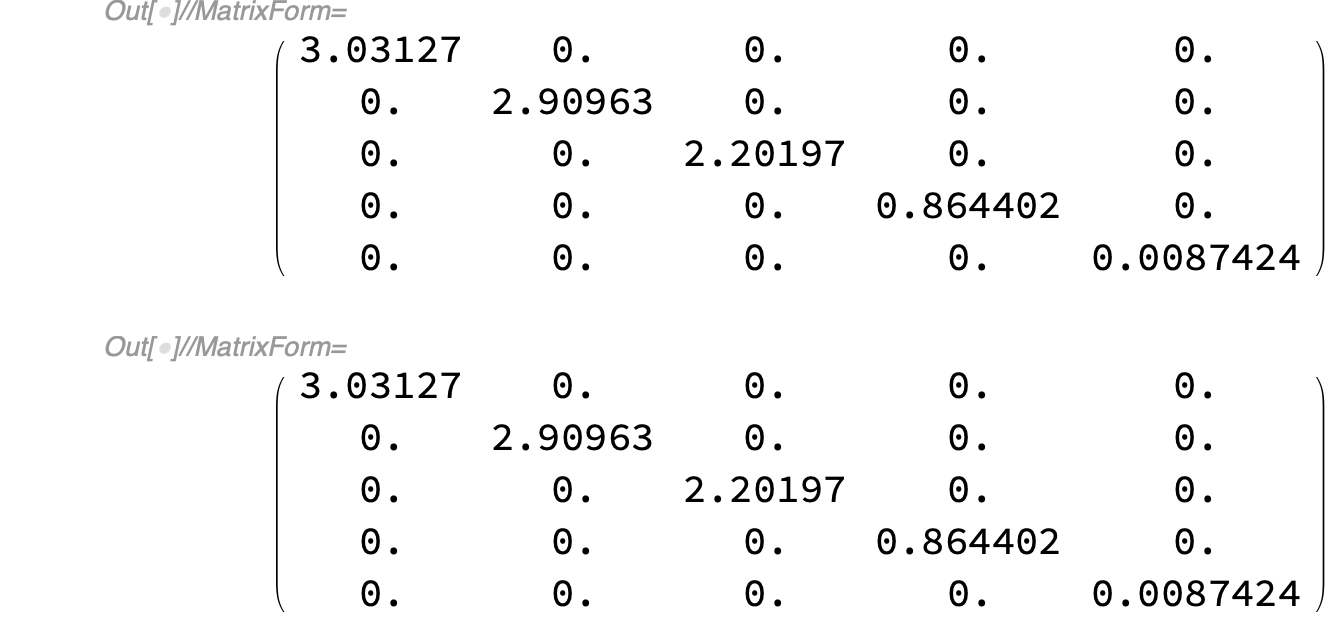
xmat . amat . xmat\[Transpose] // Threshold // MatrixForm
bmat // MatrixForm

Addendum

It should be clear that the above may be adapted to the original problem statement, amended with the suitable hypotheses:

Given two real, symmetric, orthogonally-similar matrices $A$ and $B$, not necessarily invertible, find an orthogonal matrix $X$ such that $X.A.X^t=B$.

(* set up: 5x5, rank 4 *)
SeedRandom[2];
amat = #\[Transpose] . # &@RandomReal[{-1, 1}, {4, 5}];
conj = Orthogonalize@RandomReal[{-1, 1}, {5, 5}];
bmat = conj . amat . conj\[Transpose];

(* solution *)
u1 = First@SingularValueDecomposition[amat];
u2 = First@SingularValueDecomposition[bmat];
xmat = u2 . u1\[Transpose];

Check:

Norm[xmat . amat . xmat\[Transpose] - bmat]/Norm[amat]
(*  3.12068*10^-16  *)

Since u1 and u2 are not unique, xmat is not necessarily the same as conj, and the solution xmat is unique only up to the uniqueness of the SVD. Given another solution such as conj, one can find its relationship to u1 and u2 as follows:

cj = u2\[Transpose] . conj . u1;
conj - u2 . cj . u1\[Transpose] // Norm
(*  9.36499*10^-16  *)

Addendum 2

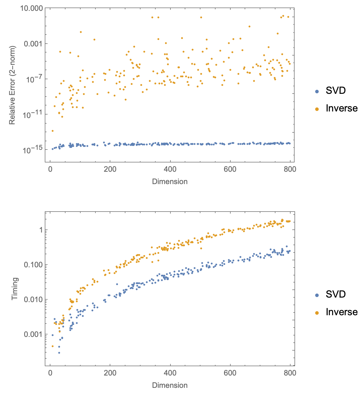
Perhaps the efficiency of SingularValueDecomposition on numerical problems is not widely appreciated. It is much more accurate than the Inverse/MatrixPower power approach and quite a bit faster. Here is a code for comparing the two methods. (Takes about a minute to run for 100 data points.)

SeedRandom[3];
(data = Transpose[#, {3, 1, 2}] &@Table[
      (* Set up: random symm. mat. of random sizes *)
      n = RandomInteger[{2, 800}];
      amat = #\[Transpose] . # &@RandomReal[{-1, 1}, {n, n}];
      conj = Orthogonalize@RandomReal[{-1, 1}, {n, n}];
      bmat = conj . amat . conj\[Transpose];
      (* SVD *)
      t1 = (v1 = Last@SingularValueDecomposition[amat];
          v2 = Last@SingularValueDecomposition[bmat];
          xmat1 = v2 . v1\[Transpose];) // AbsoluteTiming // First;
      (* Inverse *)
      t2 = (xmat2 = 
            bmat . MatrixPower[Inverse[bmat] . Inverse[amat], 1/2];) //
          AbsoluteTiming // First;
      {{{n, 
         Norm[xmat1 . amat . xmat1\[Transpose] - bmat]/
          Norm[amat]}, {n, 
         Norm[xmat2 . amat . xmat2\[Transpose] - bmat]/Norm[amat]}},
       {{n, t1}, {n, t2}}},
      {100}]) //
  MapThread[ListLogPlot[#,
      Frame -> True,
      FrameLabel -> {"Dimension", #2},
      PlotLegends -> {"SVD", "Inverse"}] &,
    {#, {"Relative Error (2-norm)", "Timing"}}] &

Inverse throws a few warnings:

...
Inverse::luc: Result for Inverse of badly conditioned matrix {<<1>>} may contain significant numerical errors.
...
General::stop: Further output of Inverse::luc will be suppressed during this calculation.

The first plot shows the relative error of the two methods on random matrices versus dimension. It illustrates the stability of the SVD method. The second shows the time each run took.